Brooks (Base) Square (BS) 101
~ The Architecture of Space-Time (TAOST)
&
The Conspicuous Absence of Primes (TCAOP) ~
VI. Appendix B
A Brief Introduction
Table of Contents
I. TAOST - the network
II. TCAOP - everything minus the network
III. Interconnectedness <---
Conclusion
References
Appendix A
Appendix B <-----
VI. Appendix B
Some new interactive additions to Brooks (Base) Square have recently been added (1/5/12, 11/5/11) s:
- Brooks (Base) Square interactive (BBSi) matrix: “BASICS” (Part I)
- An introduction movie presenting morphed images of the slideshows forming the five different presentations of the Brooks (Base) Square interactive matrix.
The entire matrix is color coded so that the visual experience of the patterns may be had without ever delving into the numbers. Nevertheless, one may grasp much of the inter-number relationships by the color alone. Morphing the images provides some bridges of continuity while also amping up the esthetic experience:
- The "BASIC" introduction to the matrix grid and the simplest, most fundamental pattern of the numbers that are formed from the main, prime diagonal are presented in a step by step fashion in three interactive slideshows (I,II and III), each presenting the same information in three distinctly different presentations;
- And, the "BASIC" introduction to the matrix grid and the simplest, most fundamental pattern of the numbers that are formed from the main, prime diagonal are presented in a step by step fashion in two slideshow movies (IV and V), each presenting the same information in two distinctly different presentations.
- Brooks (Base) Square interactive (BBSi) matrix: “ADVANCED” (Part II) will follow.
- Additional patterns (Rules 182-200):
These new additions to the Brooks (Base) Square matrix are directly...and indirectly...all about diagonals within the grid. They start with a couple of restated rules (Rules 182 and 183) taken from the original Rules 35-41. Then it jumps into new territory, exponentials in Rules 184-190. Finally, in Rules 191-200 another, deeper look at the 0/5/0 (nodes ending in 0 or 5) number patterns, and the incredible patterns found in the 1st, 2nd, 3rd, and even 4th, numbers of the sums of the Prime Diagonal (PD) numbers between these 0/5/0 nodes.
To keep these new rules in perspective, two simple lists have been generated. The first list consists of 10 General BBS Patterns and the second list is simply a subset list of one of the 10 General BBS Patterns, and is referred to as 10 General PD Patterns.
Let’s get started.
10 General BBS Patterns:
- Every Inner Grid (IG) number is generated from the PD, as IG #=PD#-PD# sequence #. Indeed, the difference, ∆, between adjacent IG numbers (i.e. 3-5-7-...) equals the ∆ between the PD #s.
- Going up or down the Horizontal Rows, the IG numbers decrease (or increase, respectively) by a ∆ of 5-7-9-... from the previous IG number.
- Going left or right across the Vertical Columns, the IG numbers decrease (or increase, respectively) by a ∆ of 3-5-7-9-... from the previous IG number.
- Going left or right across the Vertical Columns, the IG numbers increase (or decrease, respectively) by a ∆ from the PD by 1-4-9-16-25-36-....
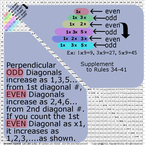
- BS Rule 182: Perpendicular ODD Diagonals increase as 1-3-5-… from the 1st diagonal number, EVEN Diagonals increase as 2-4-6-… from the the 2nd diagonal number. If you count the 1st EVEN Diagonal as x1, it increases as 1-2-3-… just like the ODD.
|
| ~click to enlarge image
|
| 182 |
BS Rule 182: Perpendicular Diagonals: ODD and EVEN
|
[ TOP ]
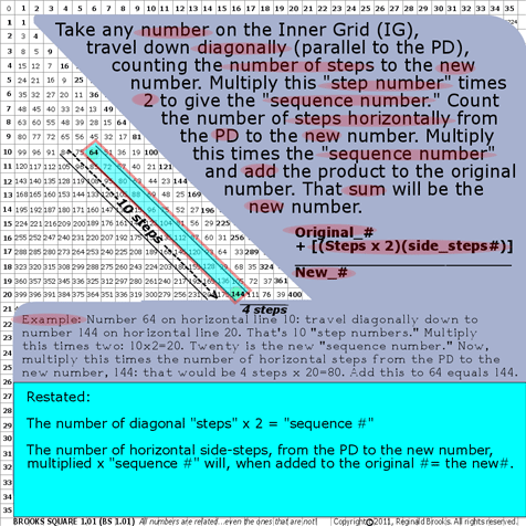
- BS Rule 183: Take any number on the Inner Grid (IG), travel down diagonally (parallel to the PD), counting the number of steps to the new number. Multiply this “step number” times 2 to give the “sequence number.” Count the number of steps horizontally from the PD (side_step #) to the new number. Multiply this times the “sequence number” and add the product to the original number. That sum will be the new IG number.
(Original IG #) + [(Steps # x 2)(side_steps #)]=New IG #
where, (Steps # x 2)= “sequence number.”
Example: Number 64 on horizontal line 10.
Travel diagonally down to number 144 on horizontal line 20. That is 10 diagonal “step numbers.”
Multiply this times two: 10x2=20. Twenty is the new “sequence number.”
Now, multiply this “sequence #” times the number of horizontal side_steps from the PD to the new number, 144: that would be 4 “steps”, so 4 x 20=80.
Add this to 64 equals 144.
Restated:
The number of diagonal “steps” x 2 = “sequence #”
The number of horizontal side_steps, from the PD to the new number, multiplied x the “sequence #” will, when added to the original IG # = the new IG #.
|
| ~click to enlarge image
|
| 183 |
BS Rule 183: Diagonal Steps between IG numbers.
|
[ TOP ]
- Rules 184-190: Exponentials:
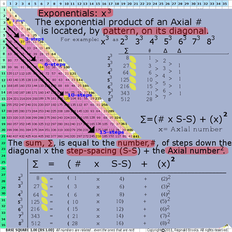
7a. BS Rule 184:Exponentials: x3
The exponential product of an Axial # is located, by pattern, on its diagonal. (That is the diagonal directly down from the Axial number.)
Example: x3: 23 33 43 53 63 73 83
The Sum, ∑, is equal to the number, #, of steps (Axial_step #) down the diagonal from Axis number “x”, times the step-spacing (S-S) plus the Axial number 2.
∑=(Axial_step # x S-S) + (x2)
where ∑=Sum (exponential product);
the step-spacing (S-S) = that difference, ∆, between subsequent diagonal numbers along that particular Axis diagonal; and,
x=Axial #
23=8=(1 x 4)+(22)
33=27=(3 x 6)+(32)
43=64=(6 x 8)+(42)
Note: the difference, ∆, distills down to 1.
|
| ~click to enlarge image
|
| 184 |
BS Rule 184: Exponentials: x3.
|
[ TOP ]
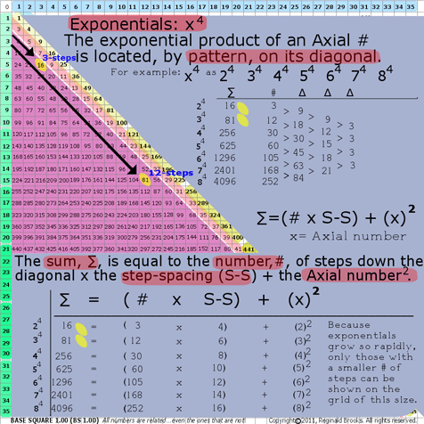
7b. BS Rule 185:Exponentials: x4
The exponential product of an Axial # is located, by pattern, on its diagonal.
Example: x4: 24 34 44 54 64 74 84
The Sum, ∑, is equal to the number, #, of steps (Axial_step #) down the diagonal from Axis number “x”, times the step-spacing (S-S) plus the Axial number 2.
∑=(Axial_step # x S-S) + (x2)
where ∑=Sum (exponential product);
the step-spacing (S-S) = that difference, ∆, between subsequent diagonal numbers along that particular Axis diagonal; and,
x=Axial #
24=16=(3 x 4)+(22)
34=81=(12 x 6)+(32)
44=256=(30 x 8)+(42)
Note: the difference, ∆, distills down to 3.
|
| ~click to enlarge image
|
| 185 |
BS Rule 185: Exponentials: x4.
|
[ TOP ]
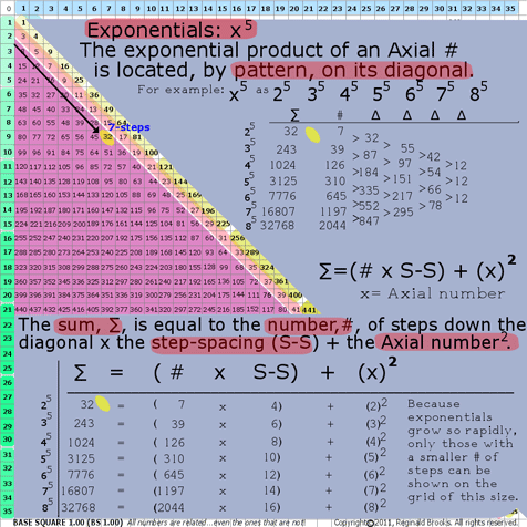
7c. BS Rule 186:Exponentials: x5
The exponential product of an Axial # is located, by pattern, on its diagonal.
Example: x5: 25 35 45 55 65 75 85
The Sum, ∑, is equal to the number, #, of steps (Axial_step #) down the diagonal from Axis number “x”, times the step-spacing (S-S) plus the Axial number 2.
∑=(Axial_step # x S-S) + (x2)
where ∑=Sum (exponential product);
the step-spacing (S-S) = that difference, ∆, between subsequent diagonal numbers along that particular Axis diagonal; and,
x=Axial #
25=32=(7 x 4)+(22)
35=243=(39 x 6)+(32)
45=1024=(126 x 8)+(42)
Note: the difference, ∆, distills down to 12.
|
| ~click to enlarge image
|
| 186 |
BS Rule 186: Exponentials: x5.
|
[ TOP ]
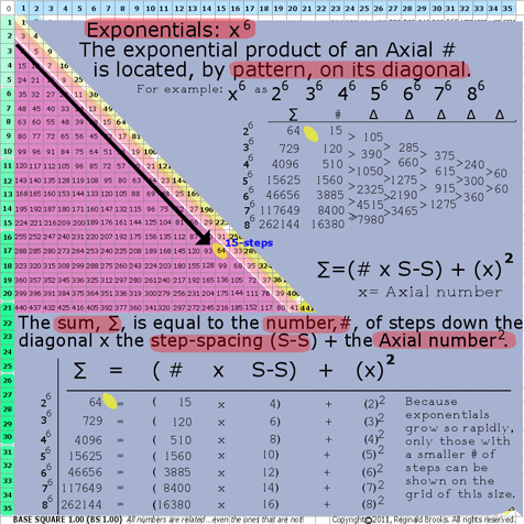
7d. BS Rule 187:Exponentials: x6
The exponential product of an Axial # is located, by pattern, on its diagonal.
Example: x6: 26 36 46 56 66 76 86
The Sum, ∑, is equal to the number, #, of steps (Axial_step #) down the diagonal from Axis number “x”, times the step-spacing (S-S) plus the Axial number 2.
∑=(Axial_step # x S-S) + (x2)
where ∑=Sum (exponential product);
the step-spacing (S-S) = that difference, ∆, between subsequent diagonal numbers along that particular Axis diagonal; and,
x=Axial #
26=64=(15 x 4)+(22)
36=729=(120 x 6)+(32)
46=4096=(510 x 8)+(42)
Note: the difference, ∆, distills down to 60.
|
| ~click to enlarge image
|
| 187 |
BS Rule 187: Exponentials: x6.
|
[ TOP ]
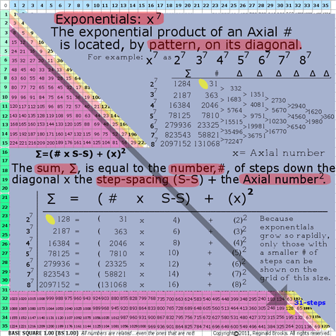
7e. BS Rule 188:Exponentials: x7
The exponential product of an Axial # is located, by pattern, on its diagonal.
Example: x7: 27 37 47 57 67 77 87
The Sum, ∑, is equal to the number, #, of steps (Axial_step #) down the diagonal from Axis number “x”, times the step-spacing (S-S) plus the Axial number 2.
∑=(Axial_step # x S-S) + (x2)
where ∑=Sum (exponential product);
the step-spacing (S-S) = that difference, ∆, between subsequent diagonal numbers along that particular Axis diagonal; and,
x=Axial #
27=128=(31 x 4)+(22)
37=2187=(363 x 6)+(32)
47=16384=(2046 x 8)+(42)
Note: the difference, ∆, distills down to 360.
|
| ~click to enlarge image
|
| 188 |
BS Rule 188: Exponentials: x7.
|
[ TOP ]
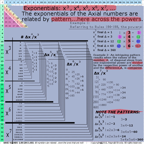
7f. BS Rule 189:Exponentials: x3 x4 x5 x6 x7 x8
The exponentials of the Axial #s are located, by pattern, across the powers.
Example 1: Referring to Rules 184-188, and the graphic for Rule 189, see that the final difference, ∆, of the diagonal step #s across the powers...x3-x4-x5-x6-... follows as 1-3-12-60-… respectively, which…when then multiplied by the exponential power value, i.e. 3-4-5-6, respectively...the product regenerates the same 3-12-60-360 final ∆ pattern as found before.
Notice the pattern within the diagonal:
x3 final ∆ =1 1x3 = 3
x4 final ∆ =3 3x4 = 12
x5 final ∆ =12 12x5 = 60
x6 final ∆ =60 60x6 = 360
Example 2: An intriguing pattern results when the values of the number, #, of diagonal steps from one exponential power are divided by the respective power of another and the difference, ∆, is compared. (Note: This is NOT division of the exponents themselves, as that would lead to subtraction, rather it is division of the diagonal steps, #, values.) See graphic for Rule 189.
Notice the pattern across the powers:
∆x4/x3: all reduce to 1
∆x5/x3: all reduce to 2
∆x6/x3: all reduce to 6
∆x7/x3: all reduce to 24
Notice the patterns!
∆x4/x3: 1 = 1
∆x5/x3: 1 x 2 = 2
∆x6/x3: 1 x 2 x 3 = 6
∆x7/x3: 1 x 2 x 3 x 4 = 24
while
3 = 3
3 x 4 = 12
3 x 4 x 5 = 60
3 x 4 x 5 x 6 = 360
|
| ~click to enlarge image
|
| 189 |
BS Rule 189: Exponentials: Across powers.
|
[ TOP ]
See Rule 190 to complete.
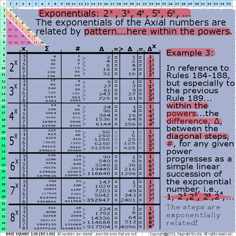
7g. BS Rule 190:Exponentials: 2x, 3x, 4x, 5x, 6x, …
The exponentials of the Axial numbers are related by pattern…here within the powers.
Example 3: In reference to Rules 184-188, but especially to the previous Rule 189… within the powers…the difference, ∆, between the diagonal steps number, #, for any given power progresses as a simple linear succession of the exponential number, i.e., 1, 21, 22, 23, 24, ….(for 2x); 1, 31, 32, 33, 34, ….(for 3x); 1, 41, 42, 43, 44, ….(for 4x); and, so on. See the graphic for Rule 190.
The steps are exponentially related!
|
| ~click to enlarge image
|
| 190 |
BS Rule 190: Exponentials: Within powers.
|
[ TOP ]
- Covertly, a simplified sub-matrix (1,2,3,...) patterned sequence grid defines the BBS matrix. See Rules 178-180 for the full exposition.
1
1 4
2 1 9
3 2 1 16
4 3 2 1 25
5 4 3 2 1 36
- This sub-matrix of linear, whole number integers can act as new fractal generators of subsequent child BBS matrixes. See below.
- Overtly, a scaffolding of 5-based (“Penta”) modules defines the BBS matrix and further informs its fractal nature. The “Penta” relationship to the BBS matrix has been previously explored as a foundation in Rules 108-153, under the I. TAOST / C. Geometrics – relationships / 3. Penta
section of the original white paper, here we are going to take a further look at this fascinating “backbone” pattern that appears to lie at the heart of the fractal nature of the BBS matrix. Here is a subset list of 10 General PD Patterns:
10 General Prime Diagonal (PD) Patterns:
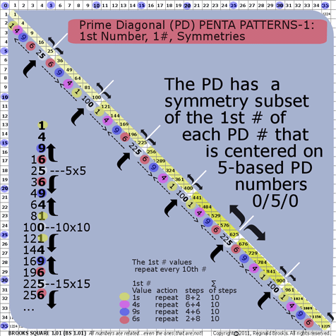
- BS Rule 191: PD-1st #s: The Prime Diagonal, PD, has a symmetry subset of the 1st # of each PD # that is centered on 5-based PD numbers ending in 0 or 5, referred to as 0/5/0 nodes. The 1st # values repeat every 10th # along the PD.
1s repeat 8+2 steps=10
4s repeat 6+4 steps=10
9s repeat 4+6 steps=10
6s repeat 2+8 steps=10
and, of course, 0s and 5s repeat every 10 steps. See graphic for Rule 191.
|
| ~click to enlarge image
|
| 191 |
BS Rule 191: Prime Diagonal Penta Patterns-1.
|
[ TOP ]
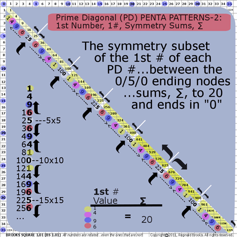
- BS Rule 192: PD-1st #s: The symmetry subset of the 1st # of each PD #…between the 0/5/0 ending nodes…sums, ∑, to 20 and ends in 0. See graphic for Rule 192
1+4+9+6=20
|
| ~click to enlarge image
|
| 192 |
BS Rule 192: Prime Diagonal Penta Patterns-2.
|
[ TOP ]
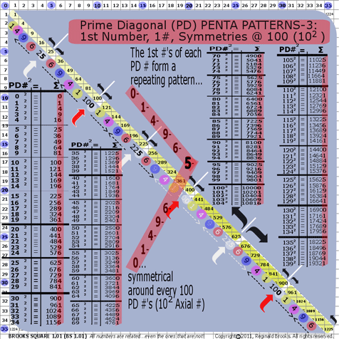
- BS Rule 193: PD-1st #s: The 1st #s of each PD # form a repeating pattern…0-1-4-9-6-5-6-9-4-1-0…symmetrical around every 100 PD #s (i.e., 102 Axial #). See graphic for Rule 193.
|
| ~click to enlarge image
|
| 193 |
BS Rule 193: Prime Diagonal Penta Patterns-3.
|
[ TOP ]
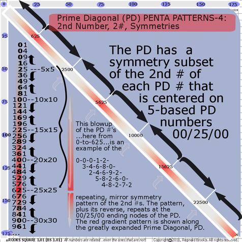
- BS Rule 194: PD-2nd #s: The PD has a symmetry subset of the 2nd # of each PD # that is centered on 5-based PD numbers 00/25/00. The blowup in the graphic of the PD #s…here from 0-to-625… is an example of the
0-0-0-1-2-3-4-6-8-0-2-4-6-9-2-5-8-2-6-0-4-8-2-7-2
repeating, mirror symmetry pattern of the 2nd #s. The pattern, plus its reverse, repeats at the 00/25/00 ending nodes of the PD.See graphic for Rule 194.
|
| ~click to enlarge image
|
| 194 |
BS Rule 194: Prime Diagonal Penta Patterns-4.
|
[ TOP ]
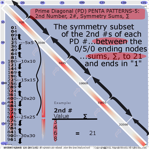
- BS Rule 195: PD-2nd #s: The symmetry subset of the 2nd #s of each PD #…between the 0/5/0 ending nodes…sums, ∑, to 21 and ends in 1.
2nd # Value: 3+4+6+8=21
2nd # Value: 2+4+6+9=21
2nd # Value: 5+8+2+6=21
2nd # Value: 4+8+2+7=21
See graphic for Rule 195.
|
| ~click to enlarge image
|
| 195 |
BS Rule 195: Prime Diagonal Penta Patterns-5.
|
[ TOP ]
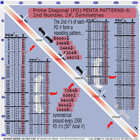
- BS Rule 196: PD-2nd #s: The 2nd #s of each PD # form a repeating pattern…
0-0-0-0-1-2-3-4-6-8-0-2-4-6-9-2-5-8-2-6-0-4-8-2-7-
2-
7-2-8-4-0-6-2-8-5-2-9-6-4-2-0-8-6-4-3-2-1-0-0-0-0…
symmetrical around every 2500 PD#s (i.e. 502 Axial #s).
See graphic for Rule 196.
|
| ~click to enlarge image
|
| 196 |
BS Rule 196: Prime Diagonal Penta Patterns-6.
|
[ TOP ]
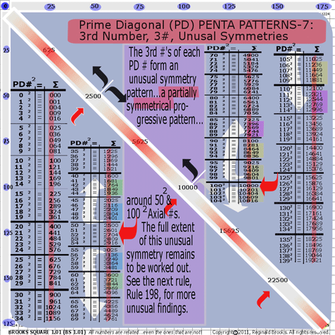
- BS Rule 197: PD-3rd #s: The 3rd #s of each PD # form an unusual symmetry pattern…a partially symmetrical progressive pattern…around 502 & 1002 Axial #s. The full extent of this unusual symmetry remains to be worked out. See the next rule, Rule 198, for more unusual findings.
1225
1296 2
1369 3
1444 4
1521 5
1600
1681 6
1764 7
1849 8
1936 9
2025 0
2116 1
2209 2
2304 3
2401 4
2500 0 -------------------->502
2601 6
2704 7
2809 8
2916 9
3025 0
3136 1
3249 2
3364 3
3481 4
3600 6
3721 7
3844 8
3969 9
4096 0
4225 2
4356 3
4489 4
4624 6
4761 7
~~~~~~~~~~~~~~~~~~~~~~~~~~~~~
7225
7396 3
7569 5
7744 7
7921 9
8100 1
8281 2
8464 4
8649 6
8836 8
9025 0
9216 2
9409 4
9604 6
9801 8
10000 0 ---------------> 1002
10201 2
10404 4
10609 6
10816 8
11025 0
11236 2
11449 4
11664 6
11881 8
12100 1
12321 3
12544 5
12769 7
12996 9
13225
See graphic for Rule 197.
|
| ~click to enlarge image
|
| 197 |
BS Rule 197: Prime Diagonal Penta Patterns-7.
|
[ TOP ]
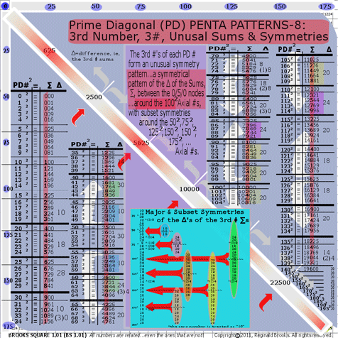
- BS Rule 198: PD-3rd #s: The 3rd #s of each PD # form an unusual symmetry pattern…a symmetrical pattern of the sums, ∑, of those #s between the 0/5/0 nodes…around the 1002 Axial #s, with subset symmetries around the 502, 752, 1252, 1502, 1752, …, Axial #s.
The four numbers...in this case, the four 3rd column numbers...of each PD # between the 0/5/0 nodes is summed and these sums, ∑, form the symmetrical patterns splaying out in opposite directions as similar progressions (not mirror symmetries).
The small rectangular inset in the lower part of the graphic shows these ∑ symmetry progressions as major and subset symmetries with considerable overlap.
See graphic for Rule 198.
|
| ~click to enlarge image
|
| 198 |
BS Rule 198: Prime Diagonal Penta Patterns-8.
|
[ TOP ]
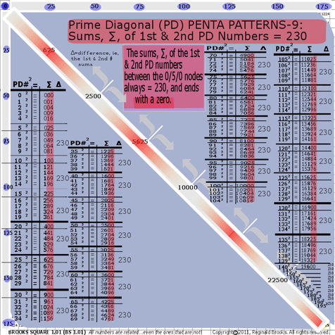
- BS Rule 199: PD-1st & 2nd #s: The sums, ∑, of the 1st & 2nd numbers between the 0/5/0 nodes always =230 and ends with a zero.
4900
5041
5184 ∑=230
5329
5476
5625
5776
5929 ∑=230
6084
6241
6400
6561
6724 ∑=230
6889
7056
7225
See graphic for Rule 199.
|
| ~click to enlarge image
|
| 199 |
BS Rule 199: Prime Diagonal Penta Patterns-9.
|
[ TOP ]
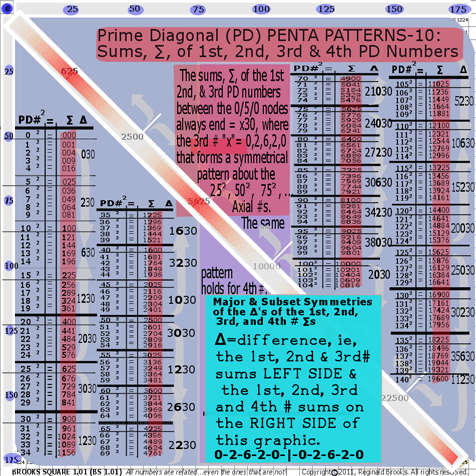
- BS Rule 200: PD-1st, 2nd, 3rd, & 4th #s: The sums, ∑, of the 1st, 2nd & 3rd PD numbers between the 0/5/0 nodes always ends = x30, where the 3rd # “x” = 0-2-6-2-0… that form a symmetrical pattern about the 252, 502, 752,1002, …Axial #s. The same pattern holds for the new sums, ∑, of the 1st, 2nd, 3rd, & 4th #s.
On the graphic, Rule 200, Major and Subset Symmetries of the sums, ∑, of the 1st, 2nd & 3rd PD # (between the 0/5/0 nodes) are shown on the lower left side of the PD. Those of the 1st, 2nd, 3rd and 4th PD # (between the 0/5/0 nodes) are shown on the upper ride side of the PD.
Both patterns follow the 0-2-6-2-0- | -0-2-6-2-0 symmetry of the 3rd #.
Example from Left side: 1st-2nd-3rd #s:
1225
1296
1369 ∑=1630 6
1444
1521
1600
1681
1764 ∑=3230 2
1849
1936
2025
2116
2209 ∑=1030 0
2304
2401
2500 ~~~~~~~~~~~~~~~~~~
2601
2704 ∑=3030 0
2809
2916
3025
3136
3249 ∑=1230 2
3364
3481
3600
3721
3844 ∑=2630 6
3969
4096
4225
4356
4489 ∑=2230 2
4624
4761
Example from Right side: 1st-2nd-3rd-4th #s:
4900
5041
5184 ∑=21030 0
5329
5476
5625
5776
5929 ∑=24030 0
6084
6241
6400
6561
6724 ∑=27230 2
6889
7056
7225
7396
7569 ∑=30630 6
7744
7921
8100
8281
8464 ∑=34230 2
8649
8836
9025
9216
9409 ∑=38030 0
9604
9801
10000 ~~~~~~~~~~~~~~
10201
10404 ∑= 2030 0
10609
10816
11025
11236
11449 ∑= 5230 2
11664
11881
12100
12321
12544 ∑=10630 6
12769
12996
13225
13456
13689 ∑=15230 2
13924
14161
14400
14641
14884 ∑=20030 0
15129
15376
15625
15876
16129 ∑=25030 0
16384
16641
16900
See graphic for Rule 200.
|
| ~click to enlarge image
|
| 200 |
BS Rule 200: Prime Diagonal Penta Patterns-10.
|
[ TOP ]
Because every 5 PD 1st #s are mirrored at 100, 400, 900, … as 1-4-9-16-25-36-49-64-81-100, i.e. the sums of every 5 PD 1st #s always end with either “0” or “5” (divisible by 0 or 5, and is the result that the 1st numbers 1+4+9+6=20). The Inner Grid, IG, #s reduce (Left->Right) as 1-4-9-16-…the sums, ∑, of any 5 Vertical IG #s will always end in 0/5 and their ∑s decrease in sequential amounts divisible by 5.
Example: 5 Vertical column #s starting with row 6:
35 32 27 20 11
48 45 40 33 24
63 60 55 48 39
80 77 72 65 56
99 96 91 84 75
__ __ __ __ __
325 310 285 250 205
325-15=310
310-25=285
285-35=250
250-45=205
Furthermore:
∑s of Vertical columns of 5 IG # decrease (L->R) by:
15 25 35 45
or
3x5 5x5 7x5 9x5
∑s of Vertical columns of 4 IG # decrease (L->R) by:
12 20 28 36
or
3x4 5x4 7x4 9x4
∑s of Vertical columns of 3 IG # decrease (L->R) by:
9 15 21 27
or
3x3 5x3 7x3 9x3
∑s of Vertical columns of 2 IG # decrease (L->R) by:
6 10 14 18
or
3x2 5x2 7x2 9x2
∑s of Vertical columns of 1 IG # decrease (L->R) by:
3 5 7 9
or
3x1 5x1 7x1 9x1
which only follows as the Vertical columns in the IG decrease (L->R) as 1--4--9--16--25 and the difference, ∆, is 3--5--7--9 (while the vertical difference, ∆, (up & down) follows as 1--2--3--…, respectively).
The 1st and 2nd #s of the PD are naturally present in the “Penta” Vertical column #s as this simply represents subtracting the PD by 5 or 10. The same is true, albeit in a slightly different way, for the 1st# present in the “Penta” Horizontal row. Again, this simply represents subtracting the PD at 0/5/0 nodes by the PD #.
Here’s the thing, the 1st #s of the PD…1-4-9-16-25-…explicitly, if not implicitly…relate linear # sequence to geometry. Remember, 12, 22, 32,…equals 1-4-9-…that is:
A=l2, where l = length and A=area.
We know that within the BBS IG, this same relationship is occurring with each and every #. Every IG # relates it’s area, A, back to the linear # that generated it.
Every # on the PD represents an area, A, of its linear #…in this case its the square of its respective Axial #.
Every # on the IG is a PD#-PD sequence # (1-4-9-…) and because the sum, ∑, of any 5 sequential group of PD #s-any 5 sequential group of PD 1st #s always ends in either 0/5, and all the IG #’s are simply a reflection of this. Every IG#=PD#-PD sequence #.
Ultimately, all this linear sequence to area geometry comes back to the “Penta” relationships.
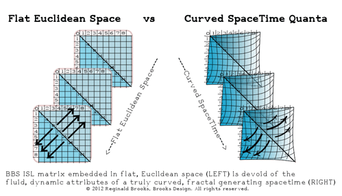
It, also, ultimately defines the fractal nature of the BBS ISL ST matrix. The ST quanta are curved. The energy density of pulse-propagating ST quanta defines the frequency...and thus the point of origin of the “0” of its defining BBS ISL ST matrix of each and every ST quanta. The higher energy (and thus frequency) pulse has a shorter wavelength and the matrix grid is correspondingly compacted...and curved. By comparison, a lower energy (frequency) pulse would have a relatively more expanded, longer wavelength grid...with all the affects of a flatter, less-curved ST quanta. This is made possible by the inherent fractal nature of the BBS ISL ST matrix. See below.
Additional Commentary
The Architecture Of SpaceTime (TAOST)...
how Brooks (Base) Square, BBS, reveals the fractal nature of the Inverse Square Law (ISL) in service to the Conservation of SpaceTime and the inevitable conclusion that dark matter = dark energy (the inverse of)
SpaceTime...that is, both space and time, interlinked as they are...falls off inverse squarely from its source, the pulse-propagated boson ST unit...which itself radiates outward at c, the velocity of light. This wave of ST propagation, occurring at the frequency of its energy relative to its wavelength, contains one Planck unit of energy and is always conserved.
When actualized at any point...that is interacting with another boson ST unit or one of its derivatives (the fermions)...the wave energy collapses to deliver it full potential payload. Constructive and destructive interference comes in to play because the boson ST units have either left, L, or right, R, handed spin 1 vectors giving:
- Spin 1L + Spin 1R = Spin 0 Higgs Boson
- Spin 1L + Spin 1L = Spin 2L Graviton
- Spin 1R + Spin 1R = Spin 2R Graviton.
In the former we have re-creation of the Spin 0 Higgs Boson from which all ST units (bosons and fermions) arise, and in the latter two, we have the creation of the left and right handed Spin 2 graviton bosons (with its associated gravitational effects, e.i. curved spacetime).
The collapse of the boson ST wave does not occur (for *bosons), or at least is only a temporary actualization of that ST point. It pulses on through this node and continues to expand outward indefinitely...temporarily actualizing itself repeatedly as it encounters other ST unit pulse waves coming from various sources.
ST unit derivatives...like energy bundles, aka mass-laden particles (fermions)...are completely susceptible to this propagating ST wave: increased density = increased curvature of ST.
Because the pulse propagating boson ST unit must maintain...that is be true to...its Conservation Laws, from its point of origin to the outer limits, any interaction(s) nearby that concentrates its energy packet must necessarily dilute its energy packet out and beyond. Because mass-laden ST units (fermion particles) are drawn into ST units with increased energy density (dark matter) and pushed away from those with decreased energy density (dark energy), there is an outward expansion of the ST Universe that is increasing by the dictates of the ISL...and the Conservation of SpaceTime. Compressing ST locally results in expanding ST distally. It follows that an increase in dark matter (compressed ST) dictates a reciprocating increase in dark energy (expanded ST).
How is BBS integrated into the physics of spacetime?
Let’s start at the beginning with a few basic concepts. The physics has been described in detail in the previous works:
- (an advanced view with a brief, but large overview and simple introduction to The LUFE Matrix)
- (a one page graphic supplement to :”Dark-Dark-Light: Dark Matter = Dark Energy” above)
- (a fresh, novel look at the joining of relativity with quantum mechanics)
- (the role of symmetry, Higgs, graviton and photon bosons in defining dark matter = dark energy )
These have all been predicated on the original L.U.F.E. and LUFE Matrix works:
- (over 200 working examples from easy on up)
- (advance, speculative journey into multiple dimensions)
- (the work that started it all )
Common notions amongst the fundamental, universal principles and laws of physics are the “constants” and the “variables.” The “constants” include:
- The Conservation Laws: SpaceTime; Velocity of Light; Energy; Mass (as mass-energy); Momentum; and, Charge.
- Particles and their identifying properties: mass; charge; spin; baryon, hadron, fermion, and lepton numbers.
- Fields, that is, the fields of energy, often expressed as force (energy per unit of time): gravitational; electromagnetic; weak; and, strong.
The “variables” being really just the result of the immersion and dynamical interplay of the “constants” within our “field of dreams”...otherwise known as physical reality.
That the Universe is a self-similar, reiterative expression of these underlying “constants” and “variables” relationships...that is, the Universe is a fractal, it is a fractal Universe...has been suggested by others, and by this author since the original “L.U.F.E.” was published in 1985.
The connection to the BBS - ISL is that the latter is the quantitative fractal template of spacetime itself...it is The Architecture Of SpaceTime (TOAST)...informing, defining and giving expression to the former, our Universe.
The “constants” within BBS are the numbers that make up the Axis, Prime Diagonal (PD) and the Inner Grid (IG). Oh...and the patterns they form! Yes! It’s all about the patterns, Baby!
The “variables” are built on and of the same BBS numbers and patterns, only as multiple BBS’s interact, the dynamics of the patterns interacting...like ripple waves on water...generate new patterns over a wide spectrum depending upon the number, intensity and distance of separation of those initiating BBS points. Substitute pulse-propagating ST units for BBS points and you have the basic vision of the fractal BBS matrix forming The Architecture Of SpaceTime.
Every unit of spacetime is pulse-propagating radially outward...quanta of spacetime being generated at a frequency and wavelength whose sum equals c, the velocity of light. Each quanta follows the ISL and its subsequent interactivity may be fully represented by the inherent pattern dynamics of the BBS matrix.
[*Bosons like the photon (spin 1), the graviton (spin 2) and the Higgs (spin 0)...all ST particles with integral (whole number) spin...are a separate class of ST particles that do NOT obey the Pauli Exclusion principle that disallows any fractional spin particle (known as fermions, like protons, neutrons, electrons, neutrinos) from simultaneously occupying the same point in ST.]
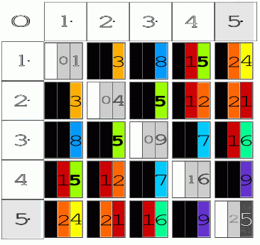
Above is a simple 5x5 matrix image of BBS.
Below, two images (Fig 5 and Fig 6) from the paper “Conservation of SpaceTime” are shown. Fuller details and the broader context can be found in this and the other reference papers cited above.
Here, we are just trying to give a very broad conceptual view of how the BBS matrix can be seen to inform The Architecture of SpaceTime.
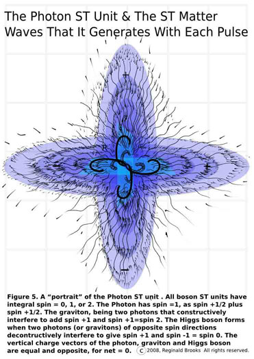
Fig 5 shows a detail close-up of the photon ST unit and its matter waves.
As it pulse-propagates into...and out of...existence, it generates the matter waves that radiate outward, obeying the ISL and effectively presenting the BBS matrix as it does so.
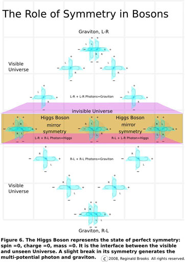
Fig 6 gives a very diagrammatic example of how this photon ST unit is derived from the super-symmetric Higgs Boson by breaking that symmetry into left- and right-handed photon bosons. These photon ST units radiate out as waves and upon crossing the wave patterns of other photon ST units have the opportunity to display constructive interference when they have the same-handed spins (either L+L or R+R) or destructive interference when the handiness of their spins is opposite. The latter simply re-instates the super-symmetry of the Higgs Boson. In the former, we have generation of the graviton...temporarily, because that is exactly what a graviton is, a Spin 2 boson formed as two photon ST unit matter waves with the same handed spin cross each other, passing through yet temporarily generating the quantum particle representing the curvature of spacetime. It is also why it is so hard to measure using conventional concepts and techniques.
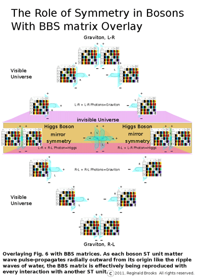
Picturing the wave ripples on the surface of water is the common example given to more easily digest the phenomenon of interference. If we now overlay the idea...represented by a smaller version of the 5x5 BBS matrix...that the energy, the force, the influence of any given pulse-propagating ST unit will, while radiating outwards, diminish inverse squarely of the distance of separation...combined with the notion that the graviton communicates spacetime curvature (gravity) by attracting mass through its local compression of spacetime, a compression...or curvature...of spacetime that decreases inverse squarely of the distance of separation from its source...effectively becoming an increasing expansion (curvature) of spacetime distally.
In the former it is the dark matter. So much local space is compressed that the curvature (gravitational pull) of the spacetime itself exceeds that accounted for by simply adding up the visible mass. And yet with distance, as the BBS matrix lays out the ISL, that curvature of spacetime is now so vastly expanded...and doing so as to quadruple for every doubling of the distance...that that part of the Universe has negative gravity, relatively, resulting from the increase in spacetime...and is the dark energy.
The dark energy thus becomes little more than the squared inverse effect of the dark matter. While the number pattern relationships of the ISL as seen in the BBS matrix quantitate this effect, it is the Conservation of Energy...i.e. all quanta of spacetime hold, and potentially deliver, one Planck unit of energy...that dictates this relationship across every scale of the Universe.
Conclusion from Dark-Dark-Light: Dark Matter = Dark Energy (the inverse of) paper:
“The irony is that the condensate of matter is light and we see it, while the fluid of which it is composed is dark and invisible. While the curvature of ST inwards toward its mass-energy seen should not exactly point to curvature outward where inflation began is the light.
For those who are in doubt, yet consider the Conservation of Energy to be inviolable, consider this:
If energy is conserved now, it must have been conserved in the past and in the future as well (that is if the notions of a past, present and future are endeared likewise).
All the energy now is the same, in amount, as all the energy at the Big Bang, both before and after inflation.
Energy disposition, that is its spatial dispersement, must likewise account for the total sum.
If the energy density fluctuates in one area, it must also fluctuate in another area or areas in an opposite manner.
If the energy density rises in one area or areas, then it must fall in another area or areas.
Force is the moderator, or interface resolution, from one energy (be it type, density or location in space or time) to another.
Force is the energy per spatial displacement.
Planck's constant, as a unit of action, is the energy per temporal displacement. It is conserved (as a constant) and as angular momentum.
If energy is conserved, then force must be conserved.
The Conservation of Force serves to uphold the Conservation of Energy.
The Conservation of Energy serves to uphold the Conservation of SpaceTime, of which it is composed of.
The Conservation of SpaceTime is built upon the velocity of light constant, c.
If the spacetime density fluctuates in one area, it must also fluctuate in another area or areas in an opposite manner.
If the spacetime density (gravitational curvature) rises in one area or areas, then it must fall in another area or areas.
If the elevated spacetime density is the Dark Matter and the depleted spacetime density is the Dark Energy then,
Dark Matter = Dark Energy (the inverse of).”Here is an example closer to home...our Sun. First, allow a squiggly waveform line...going from a point to infinity to simultaneously represent the unfolding of the BBS matrix derived ISL...that is, as the distance increases from the source point, the frequency falls as the wavelength increases (all in accordance with the ISL)...and, spacetime itself going from compression to expansion.

Anytime two or more of these progressive waveforms interact, we have the possibility of constructive or destructive interference.

Now, in the Sun, the BBS matrix-ISL source points are nearly confined to a point...nearly, but not exactly, relative to the size of the Universe. The sun’s corona runs hot! At over 200 times the temperature of the surface, the mechanism of superheating this corona plasma has defied any definitive answer. Undoubtedly, magnetism plays a hugh role...at least in accounting for the largest swings in violent activity.
Picture the core formation of the corona as follows. The corona results from a resonance band of super-interference (constructive gravitons and destructive Higgs bosons) just above the surface of the sun. The BBS matrix within the corona are the 1st harmonic resonance of the fundamental tone (frequencies) collectively of the sun proper. Changes in the density and/or angle of interference will effectively detune the resonant harmonics...perhaps to nil.
It is helpful not to forget that the BBS matrix informs the structural dynamics of spacetime...and the ST units that form it...and interchanging BBS with either SpaceTime (ST) or ST units will enhance one’s understanding of the energy, or curvature, contained therein.
In the Sun, the 1st harmonic resonance of ST curvature (a Perfect 5th), results in the entrapment and heating of a band of plasma particles exchanging high-energy photons. Is there a 2nd, 3rd, 4th,...harmonic?
In some respects, one may think of the solar corona as being the result of the “dark matter” phenomena of the Sun. Dark matter results from the concentration of compressed, local spacetime.
Since we know compressed ST here must generate expanded ST distally...where is the “dark energy” of the Sun?
Well, one can assuredly say, “Yes, it’s out there.”
Out there, but diluted in and amongst its many neighbor’s BBS matrix - spacetime contributions. Just as the Sun required a critical mass to display the corona, the Universe requires a critical mass, i.e. a critical amount of compressed spacetime in order to reveal an observable and measureable expanded spacetime...known as dark energy.
Be assured, the Conservation of SpaceTime, like the Conservation of Energy, will be the perfect accountant. All sums will add to null...zero.
Be sure to check out:The Architecture Of SpaceTime (TAOST) as defined by the Brooks (Base) Square matrix and the Inverse Square Law (ISL)
NEXT: On to
Brooks (Base) Square interactive matrix
Back to Appendix A
Page 2a-
PIN: Pattern in Number...from primes to DNA.
Page 2b-
PIN: Butterfly Primes...let the beauty seep in..
Page 2c-
PIN: Butterfly Prime Directive...metamorphosis.
Page 2d-
PIN: Butterfly Prime Determinant Number Array (DNA) ~conspicuous abstinence~.
Page 3-
GoDNA: the Geometry of DNA (axial view) revealed.
Page 4-
SCoDNA: the Structure and Chemistry of DNA (axial view).
Page 5a-
Dark-Dark-Light: Dark Matter = Dark
Energy
Page 5b-
The History of the Universe in Scalar
Graphics
Page 5c-
The History of the Universe_update: The Big
Void
Page
6a- Geometry-
Layout
Page
6b- Geometry- Space Or Time Area
(SOTA)
Page 6c- Geometry-
Space-Time Interactional
Dimensions(STID)
Page
6d- Distillation of SI units into ST
dimensions
Page
6e- Distillation of SI quantities into ST
dimensions
Page
7- The LUFE Matrix Supplement: Examples and Proofs: Introduction-Layout &
Rules
Page 7c-
The LUFE Matrix Supplement:
References
Page
8a- The LUFE Matrix: Infinite
Dimensions
Page 9-
The LUFE
Matrix:E=mc2
Page 10-
Quantum Gravity ...by the
book
Page
11- Conservation of
SpaceTime
Page
12- LUFE: The Layman's Unified Field Expose`
Page
13- GoMAS: The Geometry of Music, Art and Structure ...linking science, art and esthetics. Part I
Page
14- GoMAS: The Geometry of Music, Art and Structure ...linking science, art and esthetics. Part II
Page
15- Brooks (Base) Square (BS): The Architecture of Space-Time (TAOST) and The Conspicuous Absence of Primes (TCAOP) - a brief introduction to the series
Page
16- Brooks (Base) Square interactive (BBSi) matrix: Part I "BASICS"- a step by step, multi-media interactive
Page
17- The Architecture Of SpaceTime (TAOST) as defined by the Brooks (Base) Square matrix and the Inverse Square Law (ISL).
Copyright©2011-12 Reginald Brooks, BROOKS DESIGN. All Rights
Reserved.
(function() {
var toJsLink = function(link) {
// Check the escape conditions
if (link.href === undefined) { return; }
if (link.onclick) { return; }
if (link.className.indexOf('bkry-link-ignore') !== -1) { return; }
var handler = function(evt) {
// Look out for escape conditions
if (link.href.indexOf('#')) {
var targetUrl = link.href.split('#')[0];
var currentUrl = window.location.href.split('#')[0];
if (targetUrl === currentUrl) {
return;
}
}
// Salt in the query string argument to make sure it always gets passed around
var url = link.href;
var hash = url.split('#')[1];
url = url.split('#')[0];
var qs = url.split('?')[1];
url = url.split('?')[0];
evt.preventDefault();
window.location = url + '?' + (qs || '') + (qs ? '&' : '') + 'bkry-rewrite-links=true' + (hash ? '#' + hash : '')
return false;
};
// Bind the event handler down
if(link.addEventListener) {
link.addEventListener('click', handler, false)
} else if(link.attachEvent) { // old ie support
link.attachEvent('onclick', handler)
}
};
if (window.location.search.indexOf('bkry-rewrite-links=true') !== -1) {
// Look for new nodes
window.addEventListener('DOMNodeInserted', function(e) {
if (e.target.tagName = 'A') { toJsLink(e.target); }
}, false);
// Look for existing nodes
var links = document.getElementsByTagName('a');
for (var i = 0; i < links.length; i++) {
toJsLink(links[i]);
}
}
})();