Summary
There are two great running sums systems: One EVEN, One ODD.
EVEN
The running sums (∑) of the EVENS starts with one, adds the double of two, to that adds the doubles of four,… It’s called the Exponential Power of Two and it gives rise to the Mersenne Prime Square (MPS) and all of its constituents:
The Exponential Power of 2 is expressed as 2ⁿ: 1-2-4-8-16-32-64-128-256-512-1024-2048-4096…
The ∑ of 2ⁿ generates a sequence: 1-3-7-15-31-63-127-255-511-1023-2047-4095-8191…
You may already recognize that 3-7-31-127-8191 are not only PRIMES, but Mersenne Primes (Mp=z).
What has turned out to be of paramount importance is that ALL the numbers within the 2ⁿ sequence are important players in revealing the Mersenne Primes, Perfect Numbers (PN), ODD Complement (OC), Perfect Number Squares(PNS), ODD Complement Squares (OCS) and Complement Rectangles (CR).
How so, you might ask?
Think of this great running sums system of the Exponential Power of 2 (2ⁿ) as a subset of all the *natural whole integer numbers (WIN) that washes up as waves upon a special beach. Each wave is like a container. Simultaneously, another subset of numbers, the PRIMES, is washing up against that same special beach. Each time — and there so far have only been 51 such times — it resonates with the 2ⁿ wavelet, a Mersenne Prime is generated. And it takes interaction with ALL the “container” wavelets of the 2ⁿ to generate those 51 — so far — discovered Mersenne Primes and their embedded Perfect Numbers. These “container” wavelets are tightly interwoven within their Number Pattern Sequence(NPS) to such a degree that — while being holding spaces for the PRIMES — they present themselves over and over again as repeating parameters because that is exactly what they are based on, fractals.
The NPS of 2ⁿ generates a natural fractal. A fractal that produces bilateral (mirror) symmetry of itself with each half rigorously repeating, regenerating, reiterating itself in a self-similar manner from 1 to infinity. We call it the Butterfly Fractal 1. Every “container” wavelet and every Mersenne Prime-Perfect Number wavelet is a direct expression of the Butterfly Fractal 1.
We have seen this in the overall and we have seen this in the details, as well.
But first.
ODD
The running sums (∑) of the ODDS starts with one, adds the next ODD three, to that adds the next ODD of five,… It’s called the ODD number summation series and it gives rise to the Inverse Square Law (ISL) in that for each doubling, the sum increases by four-fold. It is the basis of the BBS-ISL Matrix (BIM).
The ODD number summation of: 1-3-5–7—9-11-13-15-17-19-21-23-25-27-29-31-…
sums to: (1)-4-9-16-25-36-49-64-81-100-121-144-169-196-225-256….
that is itself none other than the square of:
(1)-2-3-4-5-6-7-8-9-10-11-12-13-14-15-16-…
When you put this NPS together you come up with the BIM.
And then there is the BIM
The BIM, on the surface, is little more than a matrix of WINS along each axis, their squares along the diagonal, and the difference (∆) between the horizontal and vertical intersects of that diagonal informing the inner grid cells.
And yet there is so, so much more to the BIM than just illustrating the Inverse Square Law (ISL). It is so intimately inter-connected with the Pythagorean Triples that one could generate the BIM from those triples!
It is also intimately inter-connected with the PRIMES, but here in a less than obvious manner. The Goldbach Conjecture (every EVEN is composed of two PRIMES) is completely revealed to be true visually as every EVEN intercepts two -- or more -- BIM inner grid cells whose Axis coordinates are the PRIMES that sum up to said EVEN. A complete Periodic Table Of PRIMES (PTOP) is found to be "hiding" in plain sight right within the BIM.
Yet, what we are here to review is the newly discovered -- and very, very intimate -- connection of the BIM with the Mersenne Primes-Perfect Numbers and the whole Mersenne Prime Square (MPS) alluded to in the EVENS system above.
And that brings us to full circle with an important caveat: both EVEN and ODD systems are actually systems that reveal the always intimate -- and often dynamic -- relationship to their opposites. Both systems reveal as much about their opposites as themselves. The Butterfly Fractal's expression of the Exponential Power of 2 gives rise -- through the running sums (∑) -- a complete profile of ODD-number-defined PRIMES and and non-PRIMES, while the BIM itself consists of alternating ODD and EVEN numbers throughout.
We have attempted to show some of this magic!
~~~
If one considers the PRIMES as the fundamental “atoms” of the WINS, then the “Oceans of Numbers*” are the result of the interaction of the PRIMES with the "other" non-PRIMES: e.i. all EVENS are composite numbers made from the simple addition of two PRIMES (Goldbach “strong” Conjecture) and all other non-PRIME ODDS are composite numbers made from the addition or subtraction of any ODD with any EVEN or the multiplication of any two ODDs or for ODDS>7, “Every odd number greater than 7 can be expressed as the sum of three odd primes,[5]” —Goldbach’s weak Conjecture , aka the ODD Goldbach Conjecture. In this sense, the natural WINS are actually the subset of the PRIMES.
With that in mind, we can see that the PRIMES inform the WIN, the WIN informs -- through the interference resonance with the PRIMES -- the EVEN and ODD streams from which we see the Active ROWS (AR) play out on the BIM to give the Pythagorean Triples, Periodic Table of Primes (PTOP) -- responsible for the visual, algebraic-geometry proof of the Goldbach Conjecture -- and, as well as we have seen, the Mersenne Prime Squares and their embedded parameters: Mp, PN, OC, PNS, OCS, CR and the x,y and z components. The latter group being informed by that special set of doubling -- starting with quantity "1" -- that generates the "Butterfly Fractal 1" and the Exponential Power of 2.
How might one visualize this?
Instead of the renown double-slit interference, think of a series of slits corresponding to each of the PRIMES, e.i. slits of 2, 3, 5, 7, 11, 13,... all having their interference patterns co-mingling, such that at some resonant frequencies, precisely those EVENs generated interfere and sum up with those particular PRIMES to give us the Mersenne Prime-Perfect Number phenomena we find in the MPS!
As we have seen throughout, the BIM -- as presented in TPISC I, II, III, IV and now V -- is so much more than just a simple geometric matrix describing the ISL. The BIM -- and by inference, the ISL -- is fundamentally describing the structural floorplan of how space and time -- SpaceTime (ST) -- is laid out. Even something as remote and rare as the 51+ Mersenne Prime - Perfect Number intimate pairs are completely embedded within and exquisitely laid out in the BIM, one after the other. "One after the other?" you might say! Yes, one after the other when you include the necessary "containers," including "container" values for any of the 10 parameters that profile each and every MPS: p, x, x², y, y², z, z², xz, yz, and xy, a.k.a. prime, 2ᵖ⁻¹ , Perfect Number Square (PNS), y, ODD Complement Square (OCS), Mersenne Prime (Mp=2ᵖ -1), Mersenne Prime Square (MPS), Perfect Number (PN=2ᵖ⁻¹ (2ᵖ -1)), ODD Complement (OC), and Complement Rectangle (CR), respectively.
Lastly, let there be no doubt. We have only scratched the surface of the BIM here. As the template for ST formation, there remain endless possibilities -- opportunities in every sense of the word -- for future discoveries. The whole Conservation of ST via the subset Conservation Laws of Energy, Mass-Energy, Momentum, Angular Momentum, Charge,... are all predicted to have a firm basis right here within the marvelous BIM! So, get to it! Discover the BIM!
Discovery
As is often the case, upon writing up this "Summary" section, new work -- new findings -- have popped up that necessitated some deep research. Research that led us directly back to the
BIM. Findings that added -- while not taking away any of the previous finds -- some remarkable simplicity to the Mersenne Prime - Perfect Number pairing. It will be presented here in a summary form. It's called "Looking Back." Some of this was presented back in Book III: Oceans of Numbers II. More is added here. The utter simplicity of the finding more than suggests it is worthy of another look, indeed, it really does mandate a deeper look.
LOOKING BACK
When looking at the Mersenne Primes and their intimate connection with the Perfect Numbers, the tendency was to start with the Mp (z) and afterwards the PN. We might want to start the other way—with the PNs.
Imagine your on top of a waterbed — sheets, covers and bedspread — and you notice something move! What is that!
You notice — through all the coverings — that it has a shape. Maybe a square or a squarish-rectangle. You recall that a square is just a special case of rectangle — one whose sides are equal. But there are nearly square rectangles whose sides differ only slightly.
Peeling back the bedspread you find that it really is a square, but it has a line dividing it into two almost equal rectangles — both equally long, but one having its short side 1 unit larger than the other, e.i. one rectangle is 4x7 and the other 3x7, with respective areas of 28 and 21.
The bell rings as you realize 28 is a PN (1+2+14+4+7=28=the sum (∑) of 1+2+4+7+14, the factors of 28, not counting the #28 itself, and thus satisfying the definition of a PN).
The other ODD # area is a rectangle we call the ODD Complement (OC) because its ODD and it complements the PN in that they ∑ up to form a square — 28+21=49. A square we call the Mersenne Prime Square (MPS) because it is formed from squaring the long, Mp=z side of the rectangle to give, in this example, 49=7².
Thinking back to the long EVEN # and shorter ODD# sides of the PN and OC rectangles, we realize we haven’t given them a name: how abut x=EVEN and y=ODD=x-1?
Now given that info, couldn’t one just start with the x and y, get z from adding them together, and get PN=xz, OC=yz and MPS=z²? How simple.
It seems if we start with either x or y — and it doesn’t matter which in that one is simply the other +/- 1 — and get to all the other larger parameters!
So really, the connections are so direct, that knowing any one of them, one can easily derive by simple algebra or geometry (or like I like to do, by both = algebraic geometry) any and all of the descriptive parameters.
But wait, the movement continues! As you draw back the covers — leaving only the sheet —you find the PN and OC have each been further divided into a square and rectangle. The square is just the square of the short side, e.i. x² =4²=16 and y² =3²=9. We call it the Perfect Number Square (PNS) and ODD Complement Square (OCS), respectively. The rectangle, common to both, and a complement to each, is fittingly called the Complement Rectangle (CR), and in our running example equals xy=4•3=12=CR.
Doing the math, we see it fits perfectly: PNS+CR=PN and OCS+CR=OC, and PN + OC = MPS.
Once again, we only need to know x, y or z to get it ALL! (z=2x-1 and y=x-1).
But let’s go back to our initial pondering: what if we look at the x•z= PN differently?
We could start with our example — 4•7=28 — and think of it as four “7s”, i.e. four columns of 7 units each adds up to 28. This we have done extensively.
But what if we think of it as seven “4s”, instead. It really maths out to the same, but conceptually a bit different. How so?
4 4 4 4
4 4
4
Look familiar? It has the same pattern as the Butterfly Fractal 1 that we discovered was the basis for the whole Exponential Power of 2 (2ⁿ) phenomena that informs the entire Mersenne Prime-Perfective Number enterprise!
4 4 4 4 = 16
4 4 = 8
4 = 4
∑ = 28 with a Running ∑ of 4, 12, 28
The same goes for the smaller OC side: seven “3s”:
3 3 3 3 = 12
3 3 = 6
3 = 3
∑ = 21 with a Running ∑ of 3, 9, 21
The basic fractal pattern of doubling — in these cases of a cluster — exactly mimics the BF.
The full BF pattern, extensively covered in great detail, is given a quick look here:
∑ R∑
1 1 1 1 1 1 1 1 1 1 1 1 1 1 1 1 1 1 1 1 1 1 1 1 1 1 1 1 1 1 1 1 =32 63
1 1 1 1 1 1 1 1 1 1 1 1 1 1 1 1 =16 31
1 1 1 1 1 1 1 1 = 8 15
1 1 = 2 3
1 = 1 1
The simple Sums of the rows (∑) = 2ⁿ = x and x² and the Running Sums (R∑) = y and z, containers both.
One sees that each PN an OC plugs into this same BF, substituting the x or y cluster in place of the individual 1s.
Indeed, so can the MPS itself, e.i. 7²= 49 = seven “7s”:
7 7 7 7 =28
7 7 = 14
7 = 7
∑ =49 with a Running ∑ of 7, 21, 49.
What is becoming clear is that the notion of the fractal-concept-form is deeply involved in every aspect of the Mp-PN-MPS connection!
So what’s under the sheets? Ah, my friend, that remains to be seen!
~~~ ~ ~ ~ ~ ~ ~ ~~~
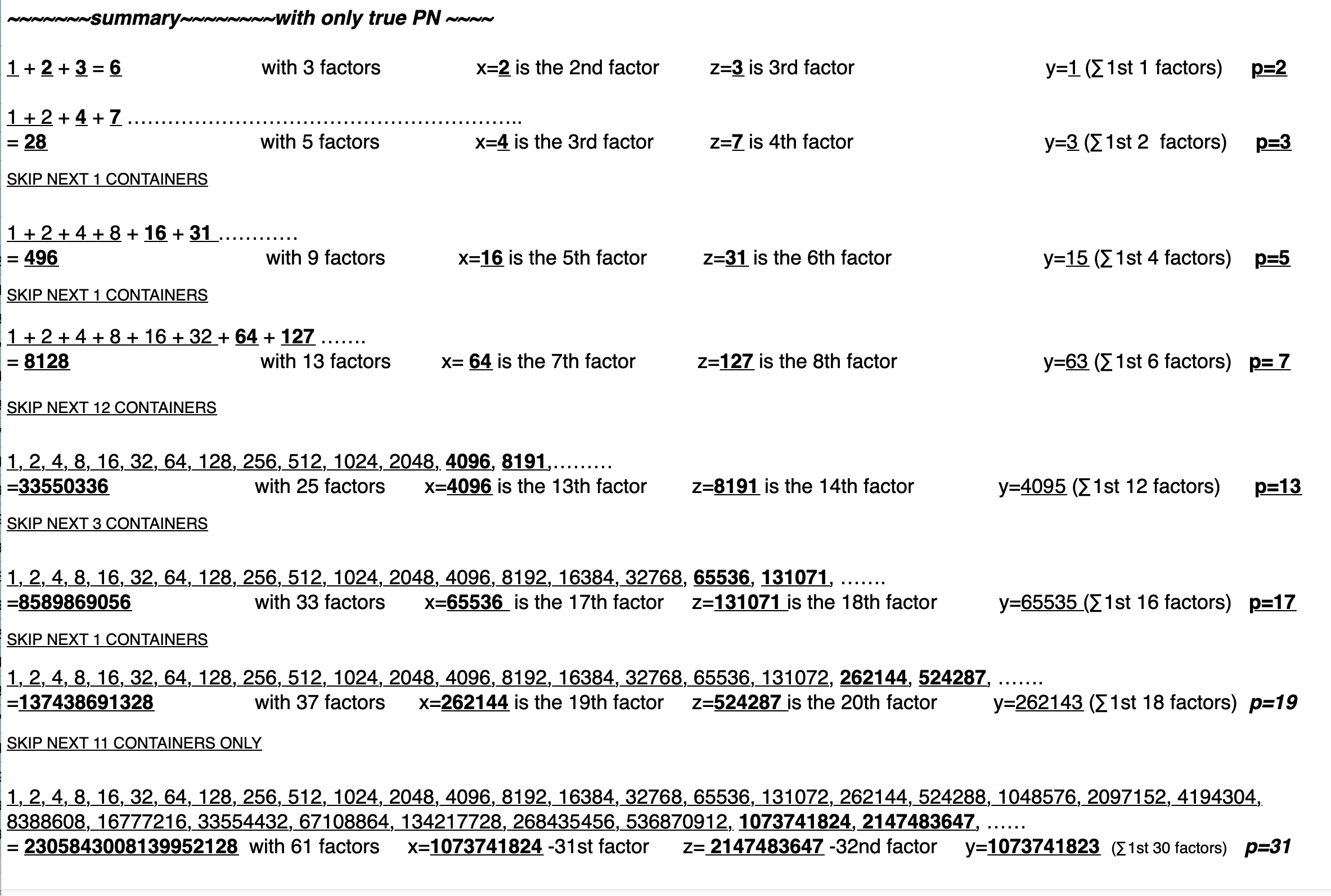
From above:
Next container: p=3 The “*p” value also indicates the number of R∑s.
∑ = 28 with a Running ∑ of 4, 12, 28 4=x 12=xy=CR 28=xz=PN
x CR PN
∑ = 21 with a Running ∑ of 3, 9, 21 3=y 9=OCS 21=yz=OC
y OCS OC
∑ = 49 with a Running ∑ of 7, 21, 49 7=z=Mp 21=yz=OC 49=z²=MPS
z OC MPS
Next container: p=4 The “*p” value also indicates the number of R∑s.
∑ = 120 with a Running ∑ of 8, 24, 56, 120 8=x 56=xy=CR 120=xz=PN
x CR PN
∑ = 105 with Running ∑ of 7, 21, 49, 105 7=y 49=OCS 105=yz=OC
y OCS OC
∑ = 225 R∑ of 15, 45, 105, 225 15=z=Mp 105=yz=OC 225=z²=MPS
z OC MPS
Next container: p=5 The “*p” value also indicates the number of R∑s.]
∑ = 496 R∑ of 16, 48, 112, 240, 496 16=x 240=xy=CR 496=xz=P
x CR PN
∑ = 465 R∑ of 15, 45, 105, 225, 465 15=y 225=OCS 465=yz=OC
y OCS OC
∑ = 961 R∑ of 31, 93, 217, 465, 961 31=z=Mp 465=yz=OC 961=z²=MPS
z OC MPS
The Running Sums (R∑) contain the MPS parameters (in BOLD)!
If we consolidate just these BOLD MPS parameters, we can better see the pattern:
∑ = 28 with a Running ∑ of 4, 12, 28 = x CR PN = x xy xz
∑ = 21 with a Running ∑ of 3, 9, 21= y OCS OC = y y² yz
∑ = 49 with a Running ∑ of 7, 21, 49 = z OC MPS= z yz z²
The only missing MPS parameter is x² and it is always found as the ∑ of x+CR=x+xy=4+12=16 above.
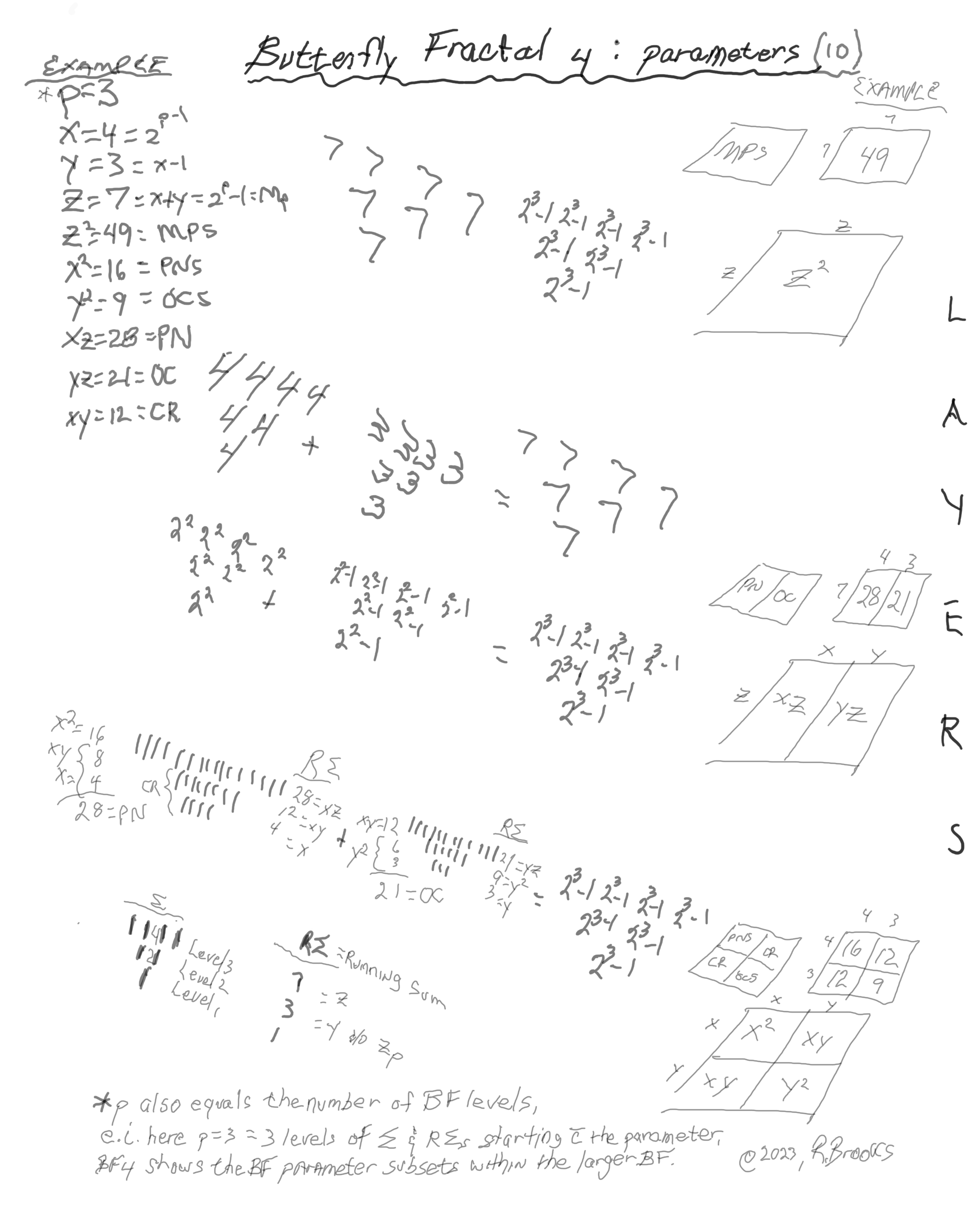
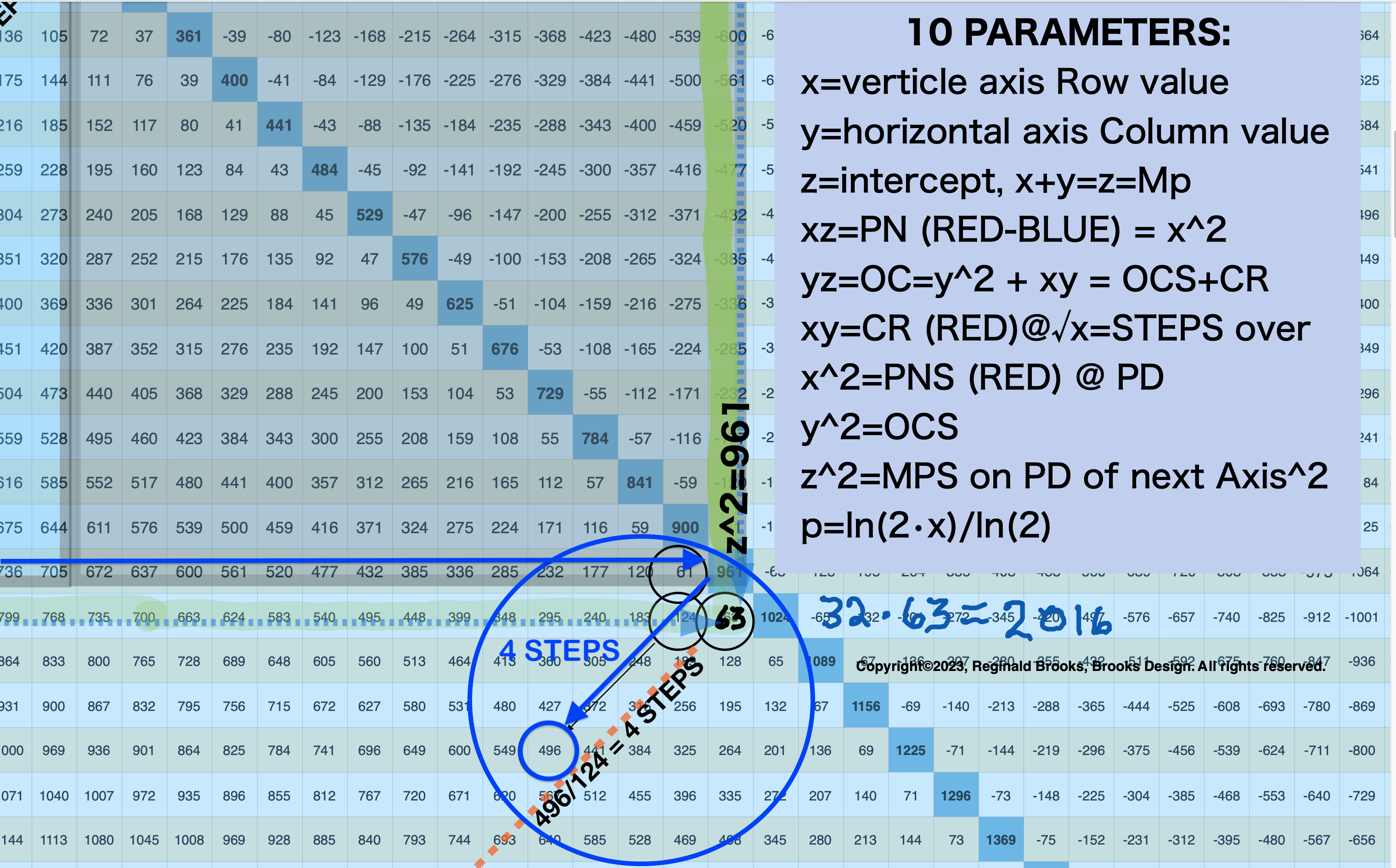
10parametersBF2.jpg. A rough schematic of what we are calling the Butterfly Fractal 4: parameters. The 10 parameters that inform each and every MPS follow this pattern. The BF4 is a subset view of the larger, initiating BF. It is based on looking at the 3 layers of the MPS: top being the MPS, middle shows the PN+OC=MPS rectangles, and the lower being the squares of the shorter sides of each rectangle -- the PNS=x2 and OCS=y2 + the CR=Complement Rectangle=xy. The "*p" value, besides denoting the exponential power of 2-1, also reflects the number of levels that this subset will show. These levels are of the same number as the parent BF1, but here, as subsets, they will reflect certain key parameters like the "x", "y" and "z" subsets with their "p" number of levels. The schematic visuals should make this clear. The following graphic with multiple MPS will expound.

BIMMPS_BFractal4.pd. Four MPS (p=2,3,4,5) as BF4 subsets are presented here. Each shows x, y, z subsets along with the original BF1 set. The 10 common parameters of any MPS are revealed in each.
Clarification
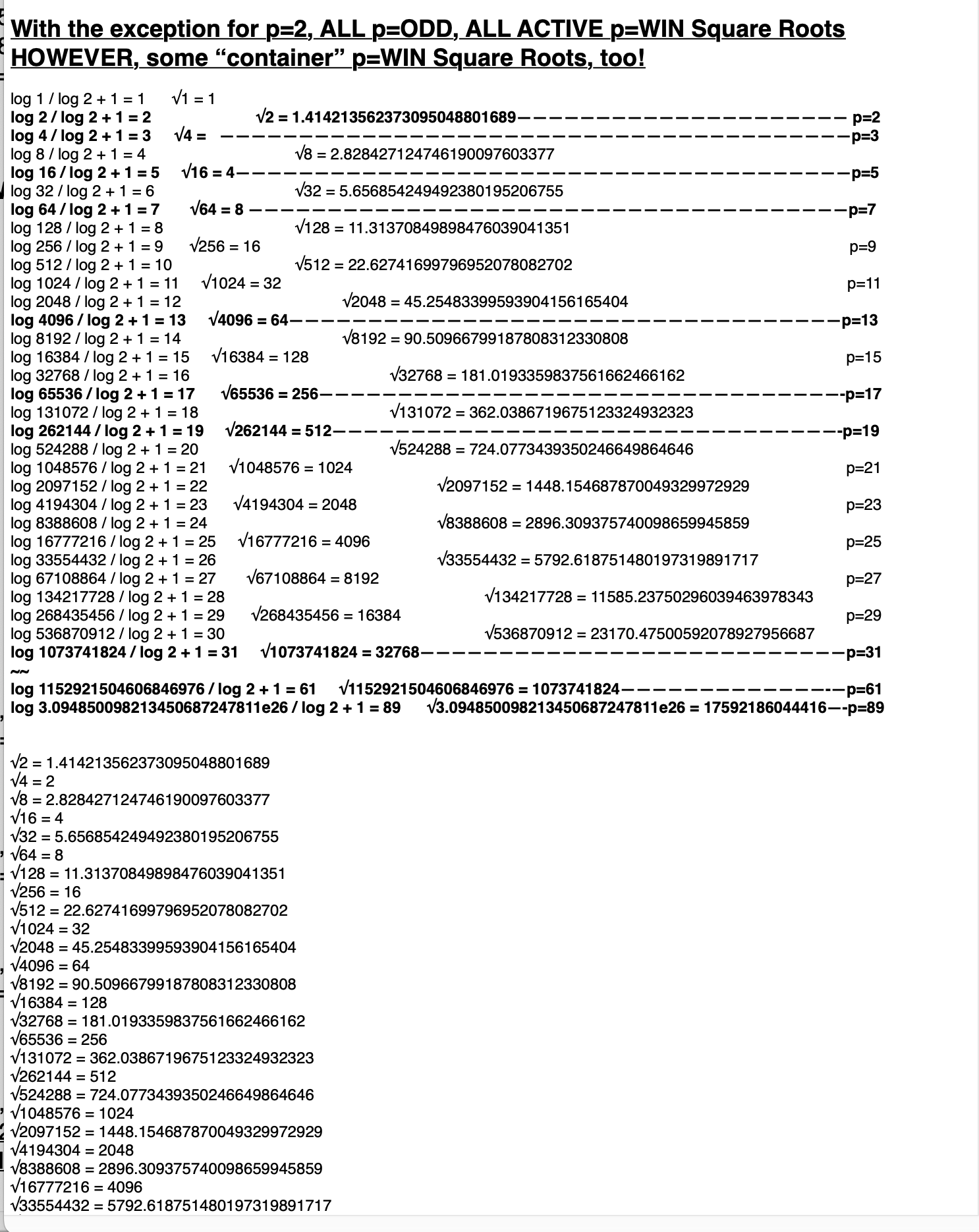
*Traditionally the “p” value=PRIME and when that PRIME is a Mersenne Prime it satisfies the Euclid-Euler Theorem:
PN=2ᵖ⁻¹ (2ᵖ-1). If we substitute x=2ᵖ⁻¹ and z=Mp=2ᵖ-1, we have PN=xz. Now, in order to “see” the Number Pattern Sequence (NPS) for the Mp-PN rarity — as there are only 51 such pairs currently known in early 2023 — we have to invoke a much larger resonate pool of values. Those of the entire pool of the Exponential Power of 2: 2ⁿ. This, of course, gives us the Butterfly Fractal 1, wherein the simple doubling of quantities, starting with 1=2⁰, 2=2¹ , 4=2² , 8=2³ , 16=2⁴ ,…, gives us all the possibilities — the resonating “containers” — within which the 51+ select Mp-PN pairs are found. Without the “containers” key parts of this NPS are lost. In order to see the whole picture — at least up to this point and view — we must invoke ALL the 2ⁿ “containers” and we do so by including within the strict “p” values, those in between “container-p”values. A strict “p” values=2-3-5-7-13-17-19-31-61-89-…. Our “container-p” values list — knowing full well that most values included are not PRIMES — includes: 1-2-3-4-5-6-7-8-9-10-11-12-13…, i.e. 2⁰ -2¹ -2² -2³ -2⁴ -2⁵ -2⁶ -2⁷ -2⁸ -2⁹ -2¹⁰ -2¹¹ -2¹² -2¹³ …. The same treatment of “containers” is in place for the other non-PRIME parameter values of Mp=z, PN=xz, OC=yz, CR=xy, PNS=x² & OCS=y², as well as x and y individually.
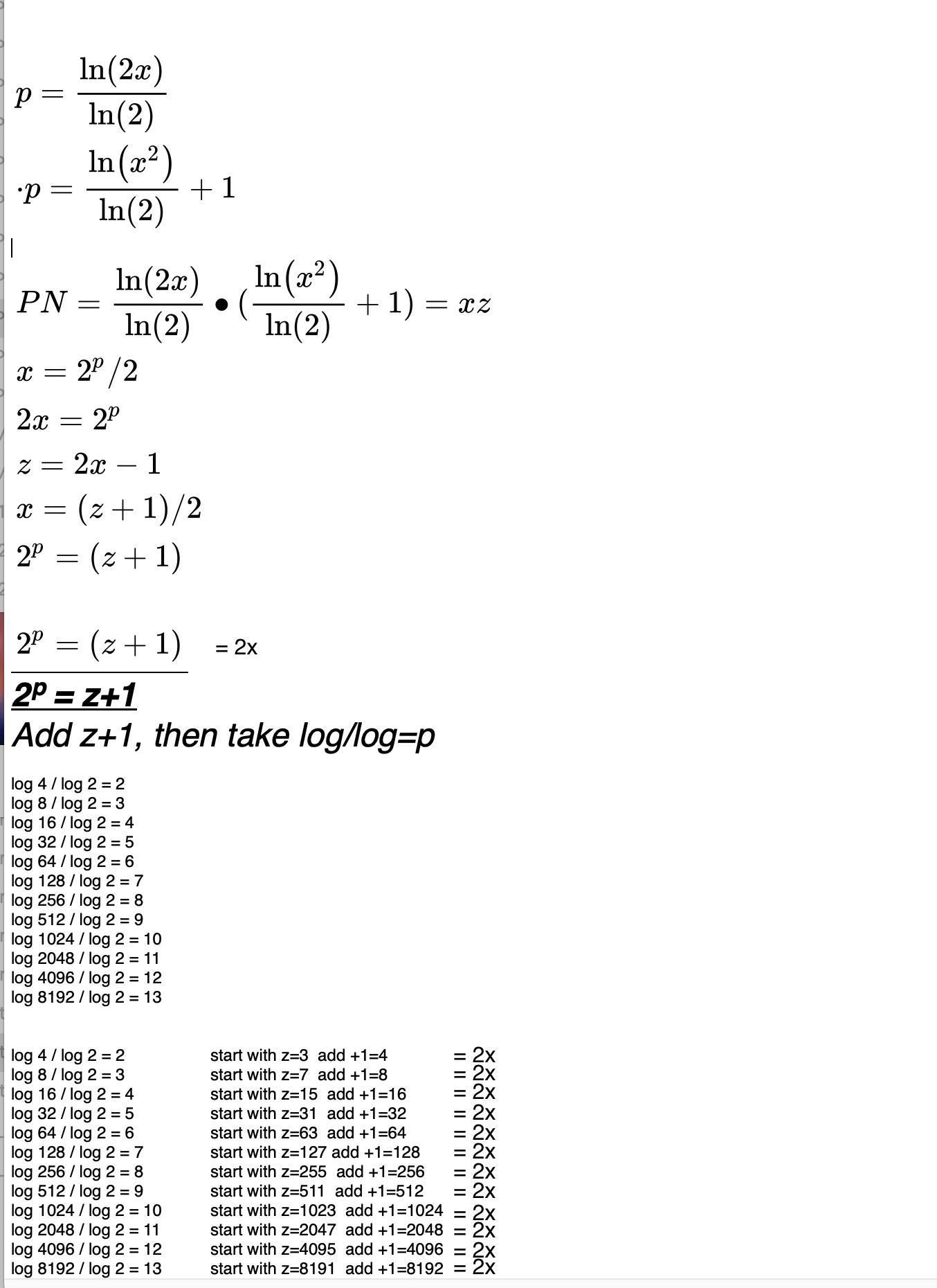
Speaking of "p" values: x=2p-1 which can be rewritten as x=2p/2. This translates to p=exponential that equals 2x. For example: let x=4, then 2x=8, and 2p solves for 8 when p=3. Another example, knowing now that 2x=2p, let's try it with x=64, then 2x=128=2p when p=7. Do remember that the "p" value also gives the number of fractal doubling levels for each respective Mp-PN-MPS set, e.i. if p=3, then there are 3 levels of R∑.
One can also solve for "p": As 2p=2x, take the logarithm of both sides, fill in the value of "x" and solve as p = ln(2x)/ln(2).
p = ln(2x)/ln(2)
If you are starting with x2 then use this:
p = [ln(x2)/ln(2)]+1

BIMMPS-150_10parametersRowAxis-xAnnot.pdf. On the BIM, this particular simplification is both especially simple in presentation, and, direct in the profile information it reveals. Effectively, "x" is now the Vertical Row Axis, "y" the Horizontal Column Axis, and "z=Mp" is the sum of the "x" and "y" coordinates, with "xz=PN" being their product. The PN then reappears in the "next" Row entry profile (see below step-by-step images). The "xy=CR" is interesting as it appears (so far) to be only on the active and TRUE x-Rows, defined as the √x=STEPS across the Row.
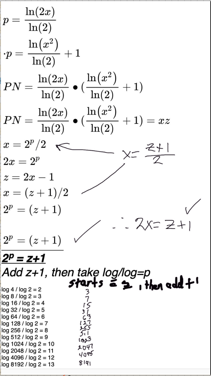
p_log_note.png. Both active TRUE and Not-TRUE "containers" are found this way. x=(z+1)/2.
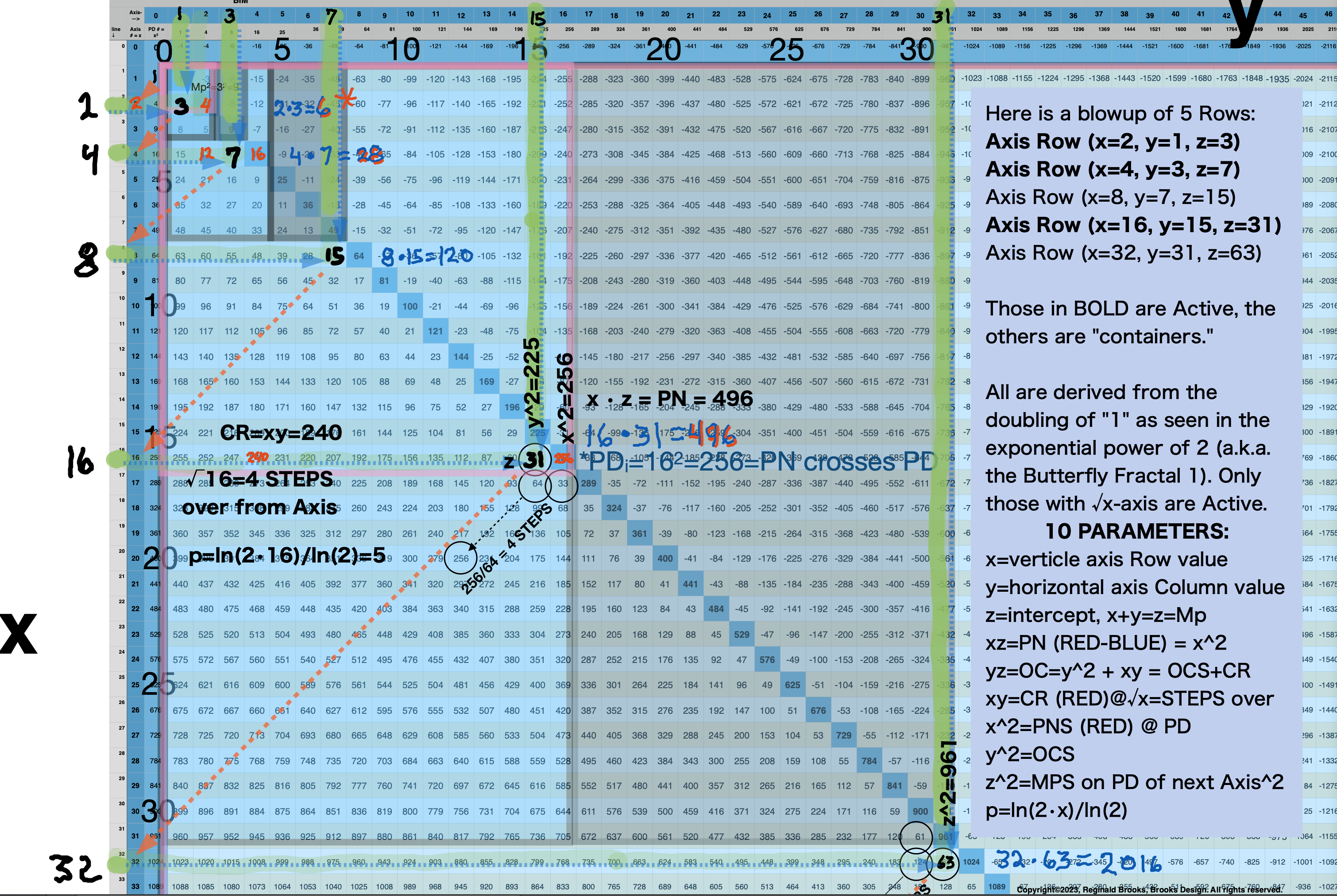
BIMMPS-150_10parametersRowAxis-xAnnotBlowup.png. The blowup series starts here. TIP: go forward and back and forth to "get" the pattern. It simply repeats in general for each subsequent "container" with the number values and STEPS expanding to fit.
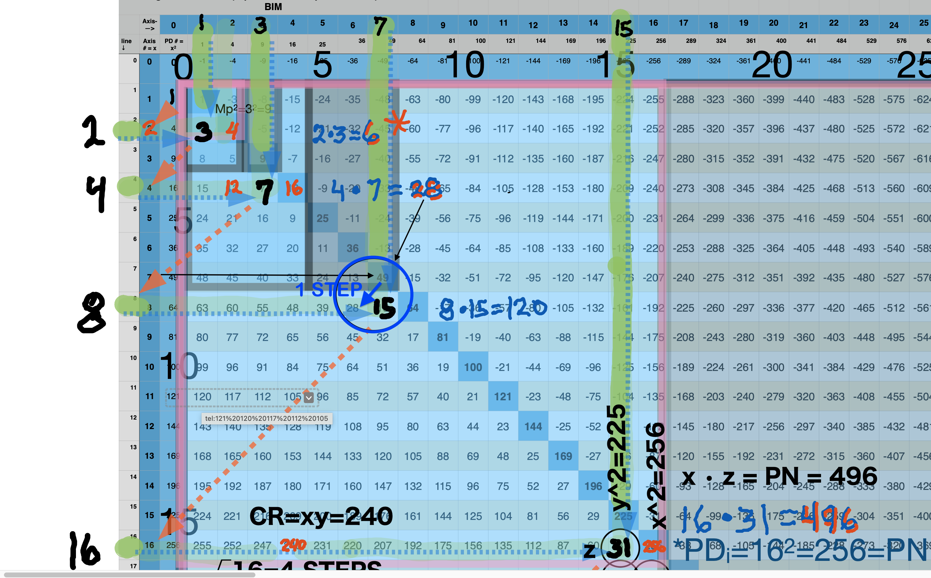
BIMMPS-150_10parametersRowAxis-xAnnotBlowup-1.png. Note that the PN=28 from Row x=4 can be found 1-Perpendicular Diagonal STEP down from the Row7 squared MPS value of 49 (on the PD). STEPS=x/8.
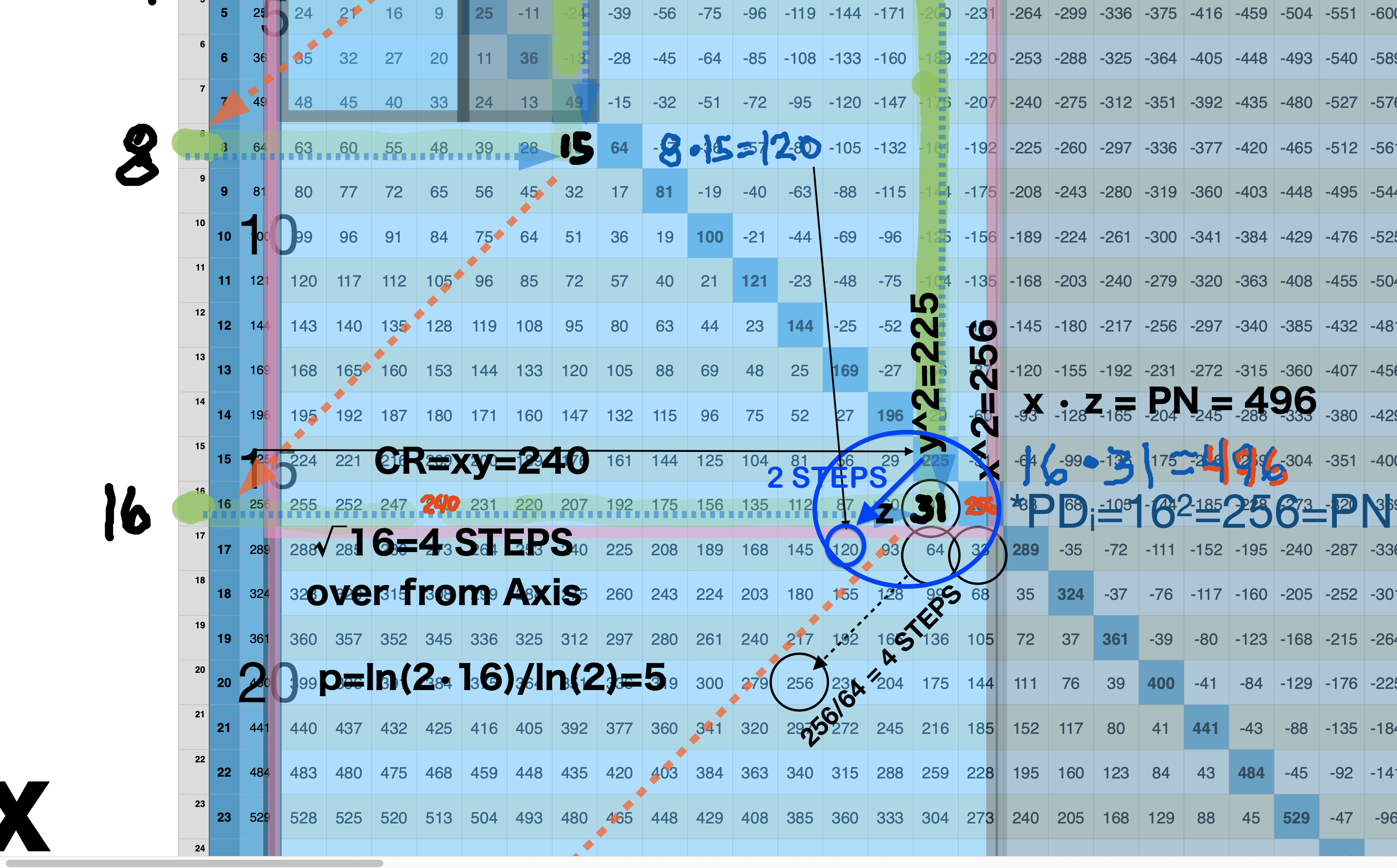
BIMMPS-150_10parametersRowAxis-xAnnotBlowup-2.png. Note that the PN=120 from Row x=8 can be found 2-Perpendicular Diagonal STEPS down from the Row15 squared MPS value of 225 (on the PD). STEPS down are 2x previous STEPS. STEPS=x/8.
BBIMMPS-150_10parametersRowAxis-xAnnotBlowup-3.png. Note that the PN=496 from Row x=16 can be found 4-Perpendicular Diagonal STEPS down from the Row31 squared MPS value of 961 (on the PD). STEPS down are 2x previous STEPS. STEPS=x/8.
BIMMPS-150_10parametersRowAxis-xAnnotBlowup-4.png. Note that the PN=2016 from Row x=32 can be found 8-Perpendicular Diagonal STEPS down from the Row63 squared MPS value of 3969 (on the PD). STEPS down are 2x previous STEPS. STEPS=x/8.
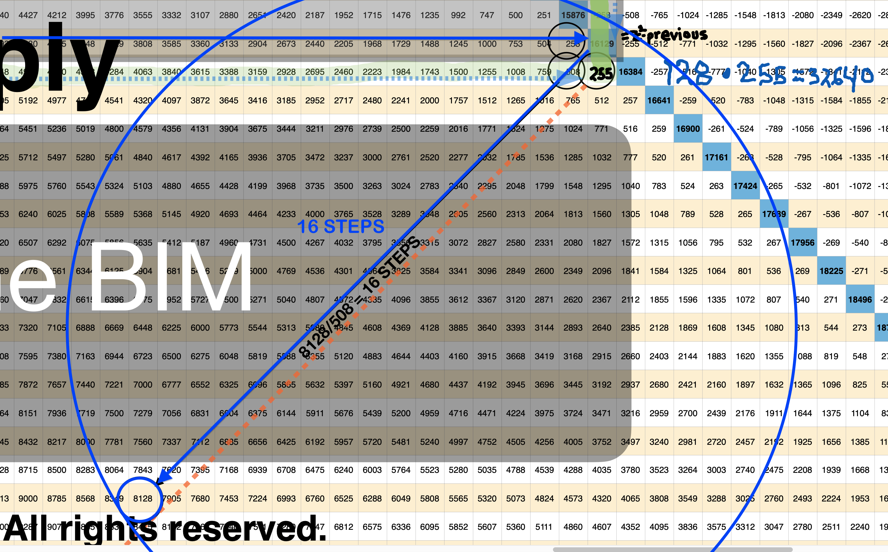
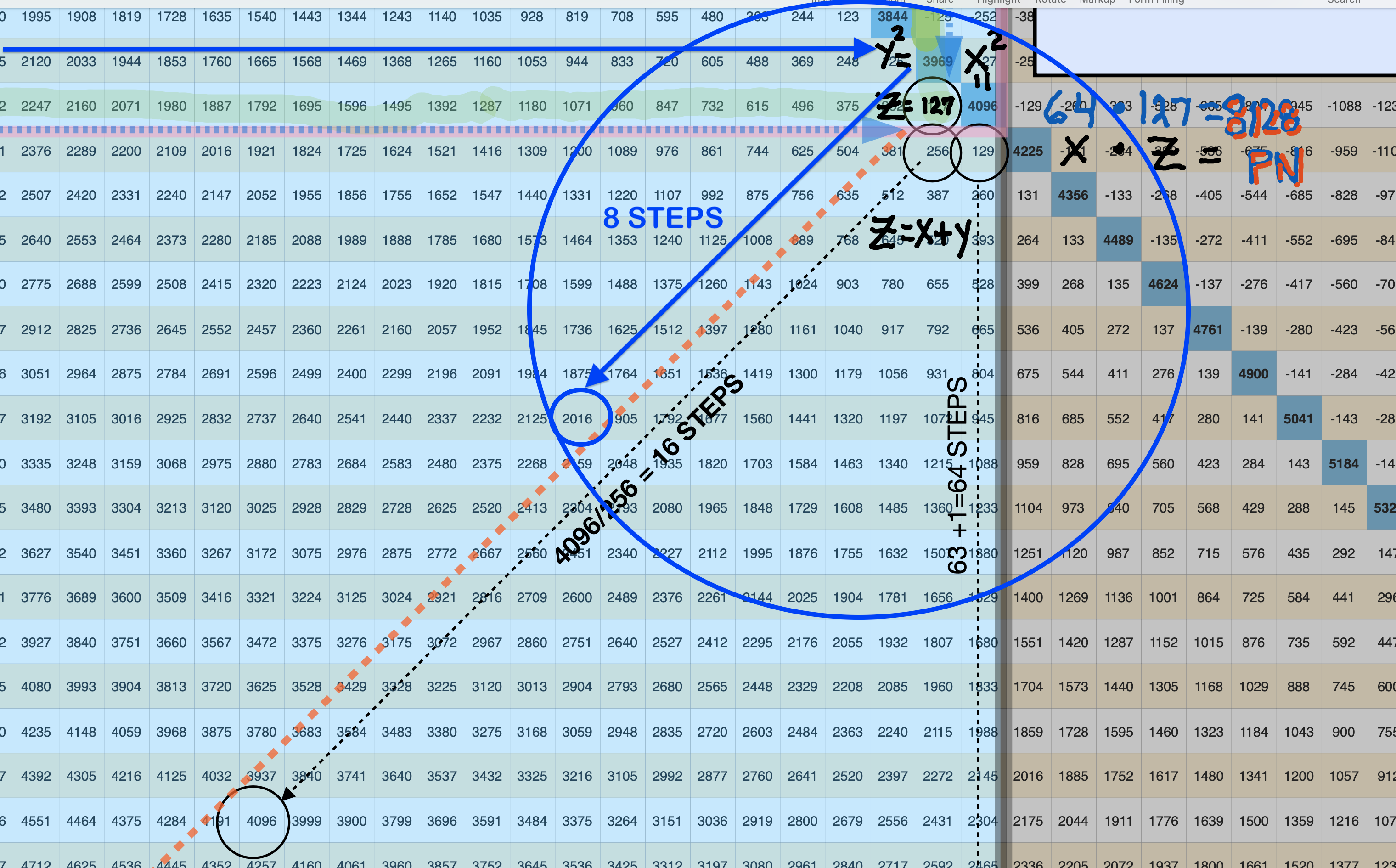
BBIMMPS-150_10parametersRowAxis-xAnnotBlowup-5.png. Note that the PN=8128 from Row x=64 can be found 16-Perpendicular Diagonal STEPS down from the Row127 squared MPS value of 16129 (on the PD). STEPS down are 2x previous STEPS. STEPS=x/8. See Table 136b-136c.
x-x-sq-p-log+.png
PNfactors-layout.png If this doesn't blow your mind, you are not paying attention!
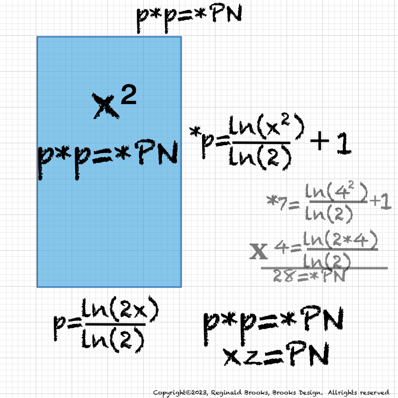
p*p=*PN.png
p=logDVDlog_*p=logDVDlog+1=xz=PN. png. p=log/log_(*p=log/log+1)=xz=PN. After adding 1 to z, enter that 2"x" value into the log equation to get the value of p. For x2, insert the squared "x" value. p*p=*PN actually translates to xz=PN. See Tables 135-137 and 124 that follows below.

BIM-MPS_3DIAGONAL_Layout2-1.pdf. Review 1

BIM-MPS_3DIAGONAL_Layout2-2.pdf. Review 2

BIM-MPS_3DIAGONAL_Layout2-3.pdf. Review 3

BIM-MPS_3DIAGONAL_Layout2-4.pdf. Review 4

BIM-MPS_3DIAGONAL_Layout2-5.pdf. Review 5

BIM-MPS_3DIAGONAL_Layout2-6.pdf. Review 6

BIM-MPS_3DIAGONAL_Layout2-7.pdf. Review 7

BIM-MPS_3DIAGONAL_Layout2-8.pdf. Review 8

Table135_solve_for_p.pdf. Tables 135-138 reveal the details.

Table135_solve_for_p-2.pdf

Table135_solve_for_p-3.pdf

Table135_solve_for_p-4.pdf

Table136_Template_p_z.pdf

Table136_Template_p_z-2.pdf

Table136_Template_p_z-3.pdf

Table137_BIM-MPS_ROWS.pdf

Table137_BIM-MPS_ROWS-2.pdf

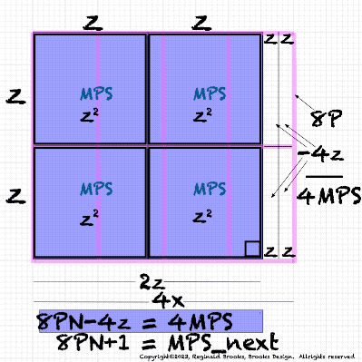
Table138_PNx4+n4.pdf. 4PN+n4=4PN+2x=PNnext.

BIM150-MPS-8PN+1=MPSnext.pdf. 8 Perfect Numbers + 1 = MPS_next.next.
GeoAREAS_4-15.gif. Summary.

Table139_8PN+1=MPSnext.pdf. 8 Perfect Numbers + 1 = MPS_next..
But wait! One discovery leads to another and we just have to show this one!
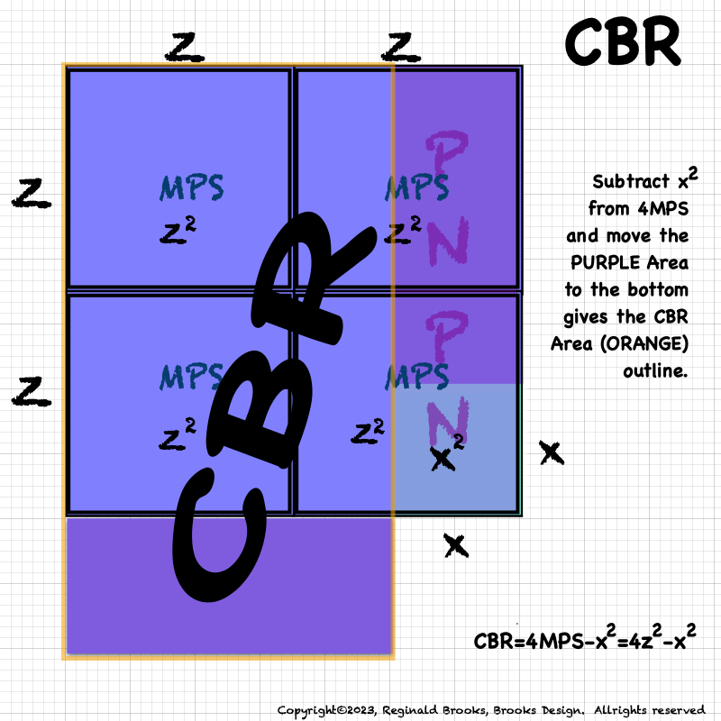
GeoAREAS_4-16.gif. Subtracting x2 from 4MPS and relocating the remainder to the bottom, forms a NEW Rectangle, the Coordinates-Based Rectangle (CBR) outlined in ORANGE.
The CBR now brings forth the fourth geometry form of the Mp-PN correlation. First was the MPS, followed by the Diamond-shaped (D-MPS) with its focus on the 10-parameters.
What happens when you look at multiples of the MPS and PN? This third geometry form combined, by layering, 8PN and 4MPS. And now the fourth form is one based on a NEW rectangle that is formed from the Axial Coordinates to give us the CBR.
What we will see in the following is that a whole new can of worms has been opened! Coordinate-Based Rectangles is a topic all by itself (covered in the Appendix). It is too important to put it entirely in basement - or is it the attic?
Briefly, we will show the natural distribution of such on the BIM, the filtering that occurs to reveal just the "containers" version of CBR and touch a bit on their significance.

BIM150-MPS-CBR-0.pdf. Template page with MPS.

BIM150-MPS-CBR-1.pdf. 1. @PD 4-8-12-16-20...a Perpendicular Diagonal will intersect with its SAME value @ Axis/4=STEPS.

BIM150-MPS-CBR-2.pdf. 2. @PD 2-6-10-14-18..a Perpendicular Diagonal intersects a PD+2•Axis value @ (Axis+2)/4=STEPS,e.i. @Axis 10: (102+2)•10=120 and 120 is located @(Axis+2)/4 STEPS=(10+2)/4=3 STEPS from the PD.

BIM150-MPS-CBR-3.pdf. 2. con'd: The BLACK lines continue back to the vertical Axis.s

BIM150-MPS-CBR-4.pdf. 3. The CBR (Coordinate-Based Rectangles) of interest, i.e. form "containers," are located where the Difference (∆) in Axial Column and Row Coordinate SUMS (∑) up to Exponential Power of 2 values. See below. The Difference (∆) in the ∆s in the same Coordinates are also Exponential Power of 2 based.
∆ in Axial Coordinates Sums (∑) and the ∆ of the ∆s:
Col Row ∑ ∆ in ∆s
3 5 8 2 2^1
6 10 16 4 2^2
12 20 32 8 2^3
24 40 64 16 2^4
48 80 128 32 2^5
96 160 256 64 2^6
192 320 512 128 2^7
384 640 1024 256 2^8
768 1280 2048 512 2^9
1536 2560 4096 1024 2^10
2072 5120 8192 2048 2^11

BIM150-MPS-CBR-5.pdf. 4. The Corners of ALL potential "containers (BLACK)" lies on the YELLOW LINE.
5. CBR Corner value ÷ 8 = ∑ of its Axial Coordinates • n, where n=x/4, e.i.
C R
46+78=124
124•4=496
496•8=3968
@16 STEPS
CBR=4MPS-x2=4z2 - x2
180=(4•49)-42 @coordinates 10•18
836=(4•225)-82 @coordinates 22•38
Col (C)=y+z Row(R)=2z+x
C•R=CBR Area
C+R=nPN where n=x/4
R-C=z+1=2x
@coordinates 46 -- 78
R-C=z+1=2x=78-46=32
x=16 y=x-1=15 z=x+7=31
z2=MPS=961 PN=xz=496
8PN=8•496=3968
4MPS=4z2=3844
C•R=CBR Area=78•46=4MPS-x2=3844-256=3588
8PN-4MPS=PN/n
3968-3844=496/4=124

Table140_Col+RowNPS.pdf. Column and Row Number Pattern Sequences (NPS).

Table141_CBR.pdf. Coordinate-Based Rectangles.

Table142_8y_series.pdf. Coordinate-Based Rectangles.
So many versions, so little time!: The next series of graphics will show, by example, how each of the geometric presentations of BIMMPS-Mp-PN corelation looks individually as well how they look when overlapped. The point here is not the details, but the larger picture of how these visualization on the BIM correlate with each other. The standard view of the MPS=PN+OC=PNS+OCS+2CR has been expanded and, you might say, refocused on particular elements such as multiples and coordinate-based presentations.

BIM20-MPPN_3Layers-0.pdf. BIM 20x20 Template page.

BIM20-MPPN_3Layers-1.pdf. Squaring the Mp=z gives the MPS=z2 Mersenne Prime Square.

BIM20-MPPN_3Layers-2.pdf. Dividing the MPS into its two slighly uneven Rectangles-PN and OC. The short side of the PN=x and that of OC=y=x-1.

BIM20-MPPN_3Layers-3.pdf. 4 MPS occupies a Square Area whose corner lands on the PD (Prime Diagonal-historically, the main or prime diagonal dividing the BIM).

BIM20-MPPN_3Layers-4.pdf. 8 PNs occupies a Rectangular Area whose corner lands outside the PD (and thus can not have its Area value read directly on the BIM).

BIM20-MPPN_3Layers-5.pdf. Here the layered overlap of the 4MPS and 8PN is shown. One can see that the 8PN Rectangle extends beyond the 4MPS by 4z. 4z= 4 Area units of 1xz. 8PN=4MPS+4z.

BIM20-MPPN_3Layers-6.pdf. This one is harder to grasp, but potentially very, very informative. Column(C) & Row(R) Coordinates = log p rectangle: p=log(2•x)/log(2) =R=×=4 and, y=x-1=C and, ×2=42=16
p=log(x2)/log(2) +1=z and z is found at intersection of C=3 & R=4, as C+R=z
R•z=PN=×z=4•7=28 and PNS+CR=Perfect Number Square + Complement Rectangle =
×2+xy=42+(3•4)=16+12=28=PN works for TRUE, Active "containers."
Not only are the "x" and "z" values derived from solving the log of p, but, with "y" = x-1, we are using the thus found "x" and "y" values as the respective Row and Column Coordinate values to locate the calculated "z" value. The full log p "rectangle" actually becomes a Square when the "x" Row value is squared.

BIM20-MPPN_3Layers-7.pdf. The log p Square-Rectangle overlaps the 4MPS.

BIM20-MPPN_3Layers-8.pdf. The log p Square-Rectangle overlaps the 8PNs.

BIM20-MPPN_3Layers-9.pdf. The log p Square-Rectangle overlaps the 4MPS and 8PNs.

BIM20-MPPN_3Layers-10.pdf. A very new finding has been the Coordinate-Based Rectangle (CBR) that matches the 8PNs Rectangle calculated value by a location on the BIM by going Diagonally down from the 4MPS corner on the PD to that value. At this Inner Grid location, one finds it to be the intersection of the Row and Column Coordinate values whose sum = nPN, where n=x/4. In this example x=4 so n=1.

BIM20-MPPN_3Layers-11.pdf. All 4 layers are combined. A direct connection between the 4MPS-8PNs-CBR layers is present.

BIM20-MPPN_3Layers-12.pdf. All 4 layers are combined. A direct connection between the 4MPS-8PNs-CBR layers is present with examples shown.

BIM20-MPPN_4Layers.mov. Video: All 4 layers are combined. A direct connection between the 4MPS-8PNs-CBR layers is present with examples shown.
Another note of clarification: y and z share the exact same “containers” and a quick look at a “container”-MPS table (Table 124) will show, their difference is one of location, i.e. the y values are staggered relative to the z values, trailing by one Row entry. The real difference between the two becomes readily apparent in the strict MPS tables: z=PRIME, y=Non-PRIME and is ÷3.
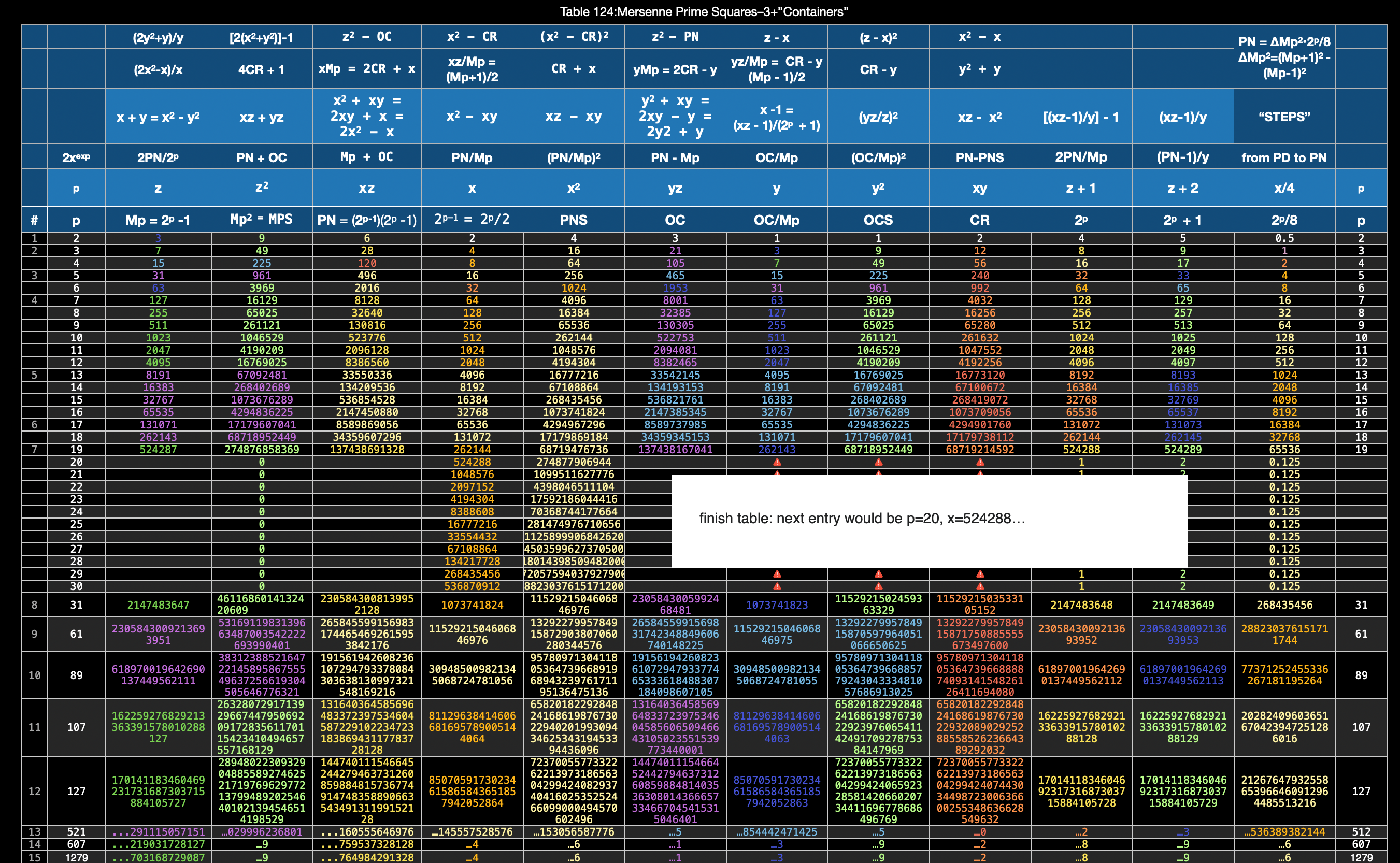
Table124_Mersenne_Prime_Squares3+containers.png
~~~~~~~~~~~~~~~~~~~~
REVIEW:
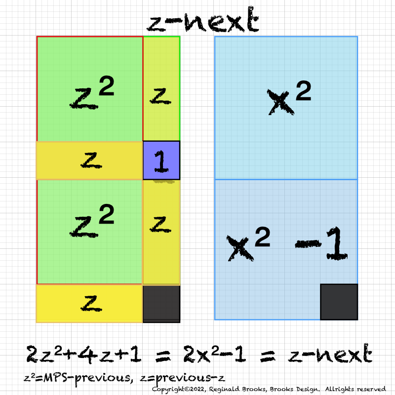
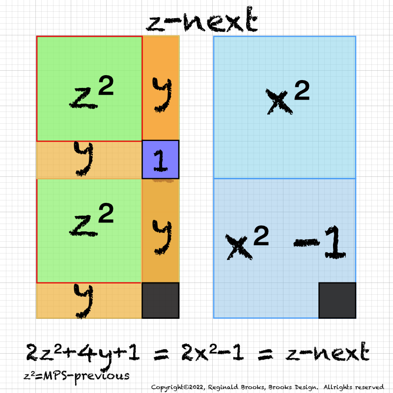
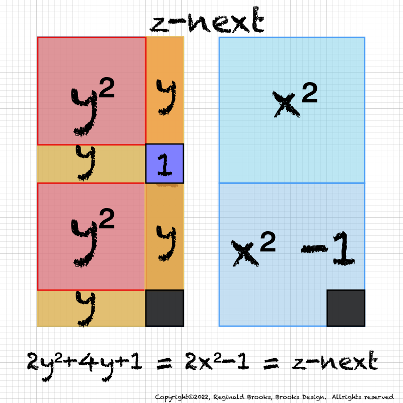
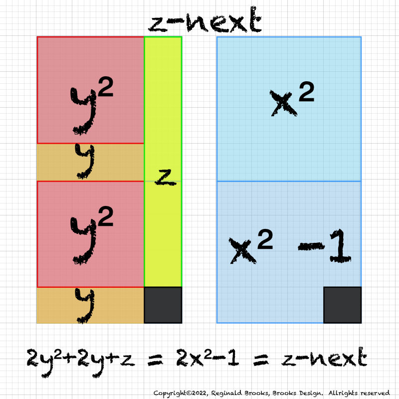
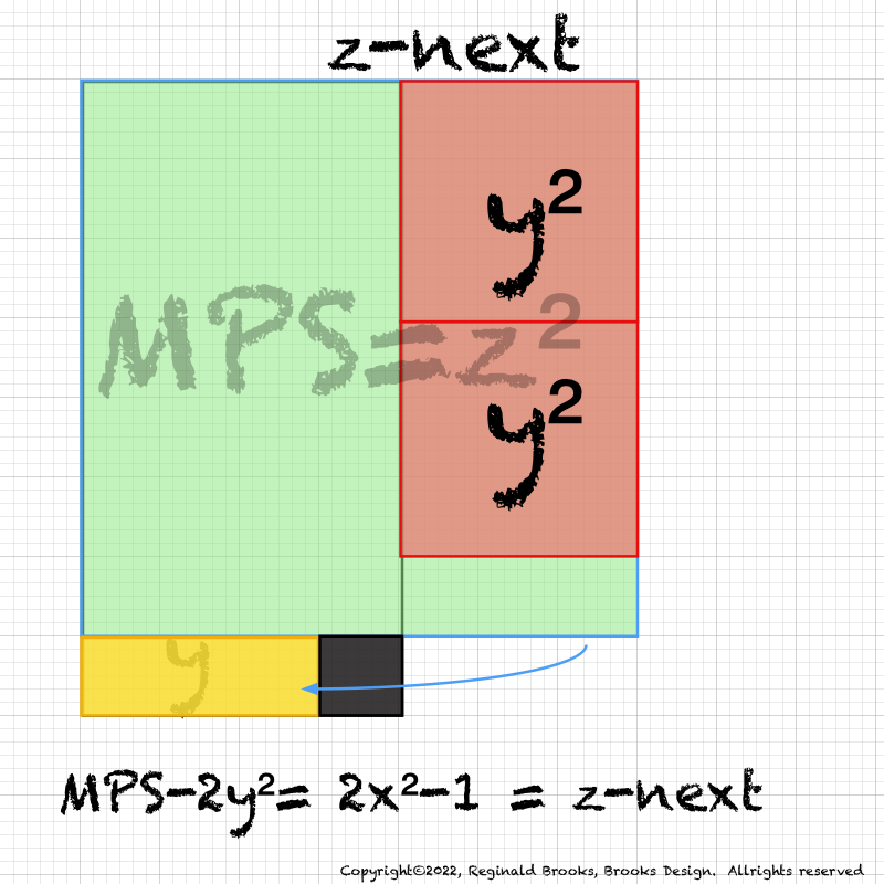
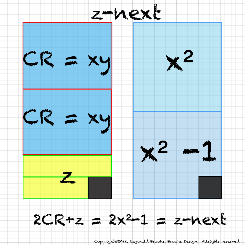
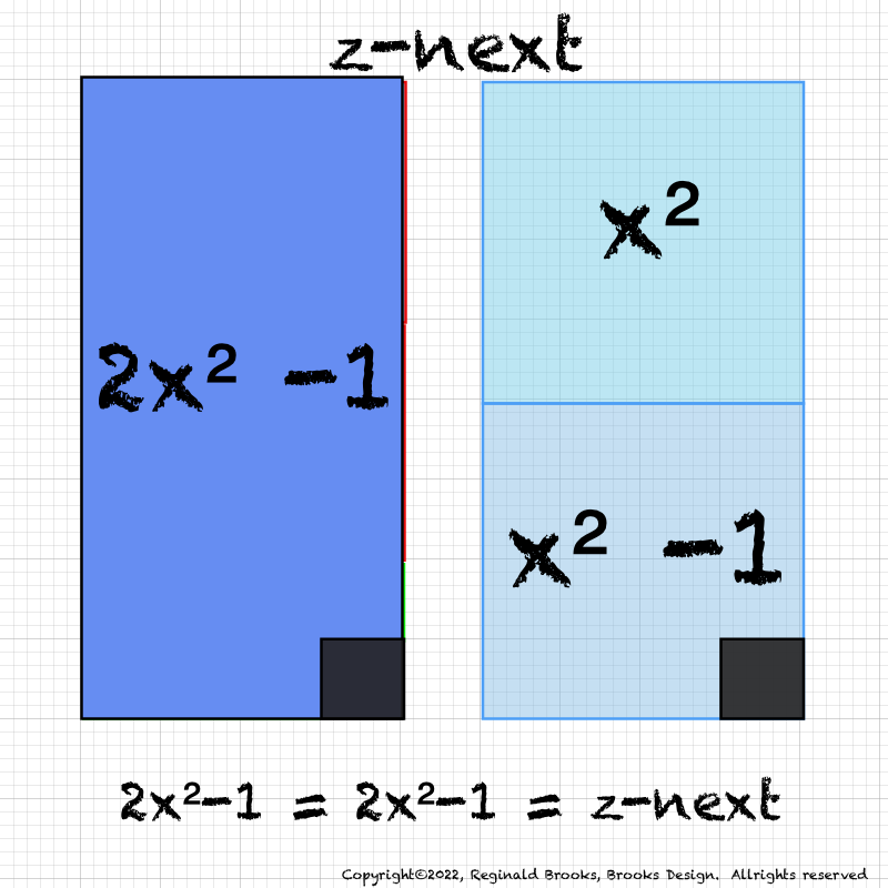
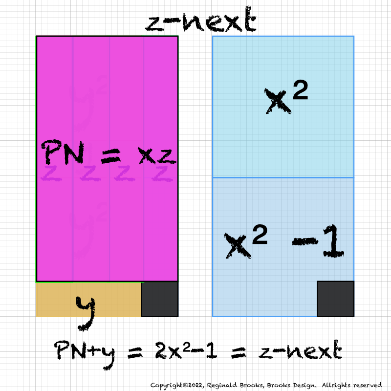
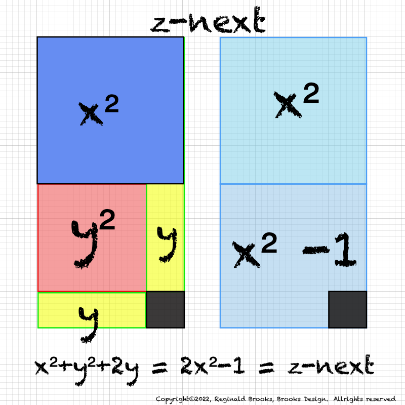
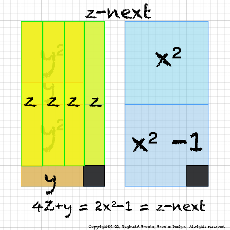
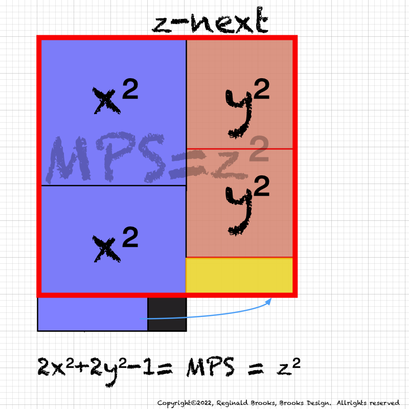
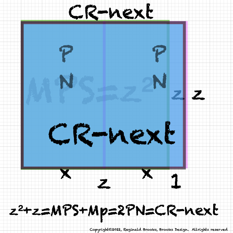
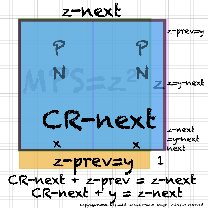
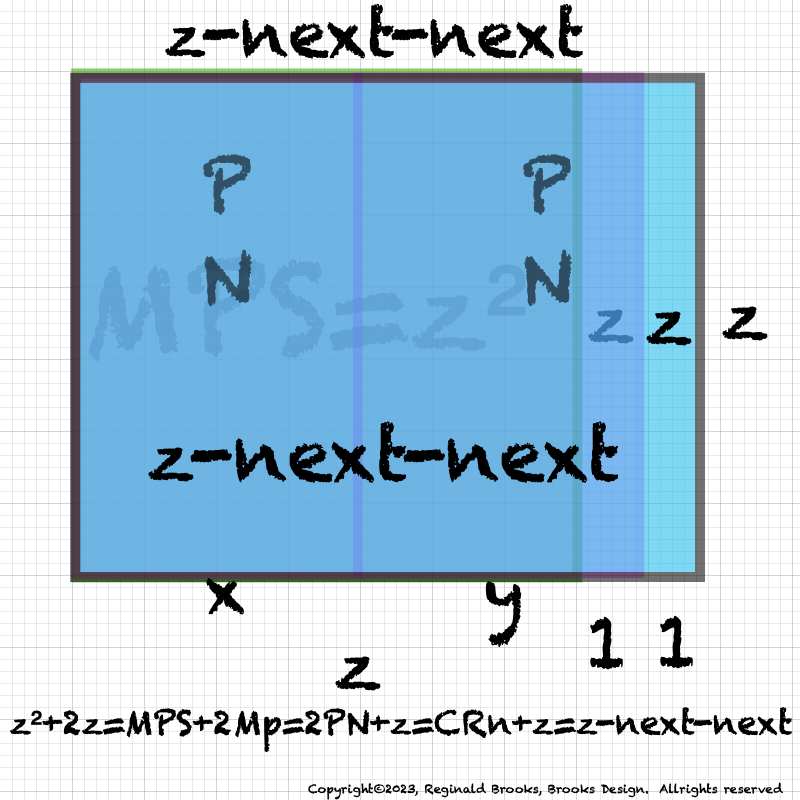
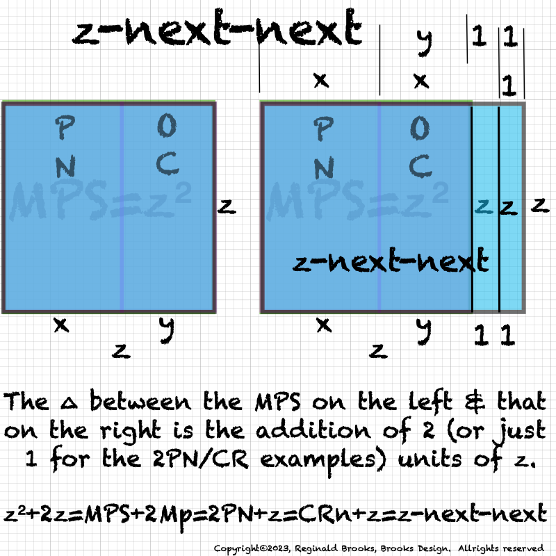
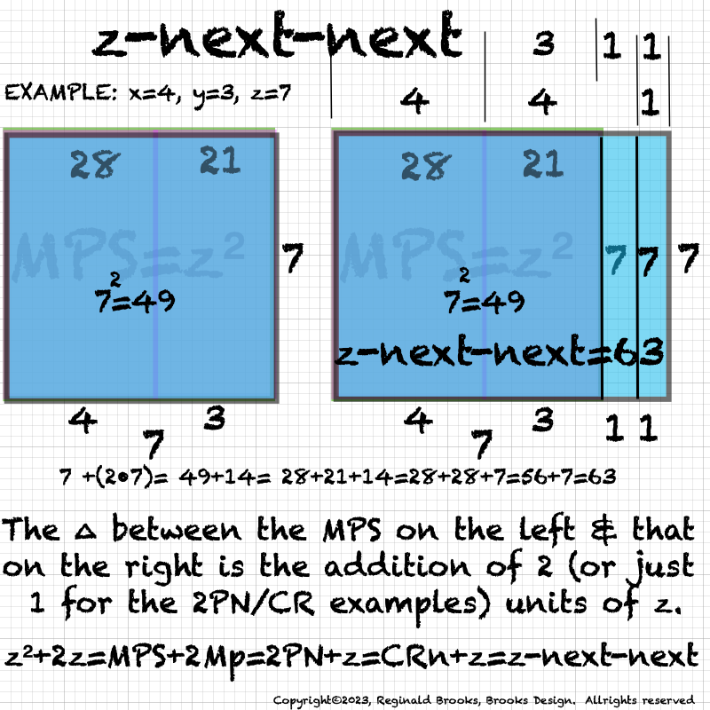
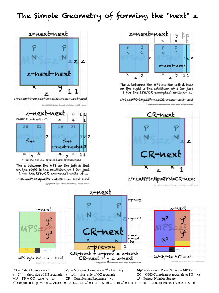
IMG_7076.PNG. What follows is highly informative visual simplification of the geometry of the MPS on the BIM series. The rectangle image (Light BLUE) on the right is a reference image of the geometry. It depicts doubling the PNS=x2 and subtracting 1, the resulting quantity (Area) equals the value of the next z=Mp. The mixed color rectangle image on the left is the one under examination. Here, 2z2 + 2y + z are equivalent to the reference on the right and thus also equal the next z = z-next. Study reaps great rewards!
IMG_7078.PNG
IMG_7079.PNG
IMG_7081.PNG
IMG_7082.PNG
IMG_7118.PNG
IMG_7085.PNG
IMG_7086.PNG
IMG_7084.PNG
IMG_7117.PNG
IMG_7083.PNG
IMG_7119.PNG

Geometry_z-next_AREAS.pdf
Tables often contain enormous amounts of data and their connections to each other. While "Tables" will be presented in a later section, Table 132a-e is worth a look now. Before resolving the geometries presented above, one connection after another of one piece of data tied to another kept coming up. It was only after placing it in table form did the more obvious solutions we see above come forth.
It is also that within the tables one sees the absolute requirement that ALL the "containers" be accounted for and included. The Number Pattern Sequences (NPS) of the MPS, Mp and PN parameters are dependent on this inclusion. And yes, this does mean including "p" values that are NOT Prime! That is the irony of the Primes to the Non-Primes, their NPS is not -- in any sense of the word -- obvious when treated as a separate group, but revealed within the larger set. One of the single most poignant revealations research on the Primes has brought out!
Speaking of "p" values: x=2p-1 which can be rewritten as x=2p/2. This translates to p=exponential that equals 2x as shown in the Tables 132 below. For example: let x=4, then 2x=8, and 2p solves for 8 when p=3. Another example, knowing now that 2x=2p, let's try it with x=64, then 2x=128=2p when p=7. Do remember that the "p" value also gives the number of fractal doubling levels for each respective Mp-PN-MPS set, e.i. if p=3, then there are 3 levels of R∑.
One can also solve for "p": As 2p=2x, take the logarithm of both sides, fill in the value of "x" and solve as p = ln(2x)/ln(2).
p = ln(2x)/ln(2)

Table132a_next_z-.pdf

Table132b_next_z.pdf

Table132c_next_z&x.pdf

Table132d_next_2PN=CRnext.pdf

Table132e_next_2PN=CRnext_2CR.pdf
In the meantime, here is another tidbit:
GeoAREAS_4-13.png
GeoAREAS_4-14.png
GeoAREAS_4-15.png
GeoAREAS_4-16.png
GeoAREAS_4-17.png
Geometry_z-next_AREAS-2.gif
In the meantime, here is another tidbit:
What happens when you mix it up just a bit, leaving all other parameters in tack? What if y equals x+1, as y=x+1, instead of its real value of y=x-1?
In our example from above, x=4 and y previously equals 3, but now let y=x+1=4+1=5.
The yz=OC=5•7=35
Then PN + OC = 28+35=63
A smaller example, MPS=9, Mp=z=3, PN=xz=2•3=6 and the original OC=yz=1•3=3. Now change y from 1 to 3, then:
The yz=OC=3•3=9
Then PN + OC = 6+9=15
A larger example, MPS=225, Mp=z=15, PN=xz=8•15=120 and the original OC=yz=7•15=105. Now change y from 7 to 9, then:
The yz=OC=9•15=135
Then PN + OC = 120+135=255
A larger yet example, MPS=961, Mp=z=31, PN=xz=16•31=496 and the original OC=yz=15•31=465. Now change y from 15 to 17:
The yz=OC=17•31=527
Then PN + OC = 496+527=1023
What is happening here? These skewed results nevertheless offer some interesting results.
The 15–63–255–1023 and the next one would 4095, are the y and/or y-container values!
A deep dive into the "Tables" section in the Appendix may help sort this one out.